Generate multifile references for HYCOM using kerchunk

HYCOM data on AWS Open Data are stored in 63,341 NetCDF 64-bit offset files. The data in these files are stored as short integers with scale_factor and add_offset, but because these are not NetCDF4 files, there is no compression and no chunking. Each file contains one time step of data.

We generate references for each file, and use kerchunk.utils.subchunk to create virtual chunks so that each vertical layer is treated as a chunk. For this uncompressed data, the byte-ranges are the same for each file, so we only need to create references for one file and then clone that for all the files, changing only the URL and the time value.

---

Overall workflow

This notebook demonstrates a kerchunk workflow for converting many NetCDF files into a virtual Zarr dataset without copying the data. The goal is to make large collections of model output (like HYCOM) behave like a single cloud‑optimized dataset.

Key idea: Kerchunk builds references, not data

• The process reads NetCDF metadata.
• It records where each variable and chunk lives inside the file.
• The result is a mapping (JSON or Parquet) kerchunk → byte range in original NetCDF file

This means:

• No data duplication
• Very fast dataset assembly
• Works well with cloud storage

It enables:

• cloud‑native access
• fast subsetting
• scalable analysis

The mental model:

NetCDF files
      ↓
kerchunk reference generation
      ↓
combined reference dataset
      ↓
virtual Zarr dataset
      ↓
xarray.open_dataset()

Step 1. Build a template reference dictionary used across files

The files need to be structurally identical. For example:

temperature(time, depth, lat, lon)

Each file needs to contain:

• the same variables
• the same grid
• the same dimensions
• a different time slice

The template dictionary defines the dataset schema. We will update the data file urls (to the netcdfs) in that dictionary.

Step 2. Create a list of dictionaries

From the template, update the data file urls (to the netcdfs) in that dictionary to create a dictionary for each file.

Step 3. Write the data dictionary to parquet

Instead of saving one large JSON reference file (which is an option), this workflow stores references in Parquet.

• faster reads
• better scalability
• efficient metadata access
• works well with distributed systems

Do all NetCDF files need to have the same structure to create a virtual Zarr dataset?

In most cases, yes — the NetCDF files used to build a virtual Zarr dataset (for example with kerchunk, VirtualiZarr, or MultiZarrToZarr) must have a consistent structure. The most important requirements are:

1) Variables must be consistent The same variables should exist in each file (e.g., temperature, salinity). If a variable appears in some files but not others, the virtual dataset may fail to build or behave unpredictably.

2) Dimensions must be compatible Dimensions like lat, lon, and depth usually need to be identical across files. The dimension along which files are combined — typically time — can differ in length, because that is the axis being concatenated.

3) Coordinate systems must match

• Same latitude and longitude values
• Same vertical levels
• Same projection or reference system

4) Chunking and compression can differ These are storage details and usually do not need to match. Kerchunk reads the metadata and builds references regardless of how the data are chunked internally.

Let’s get started!

from kerchunk.netCDF3 import NetCDF3ToZarr
from kerchunk.combine import MultiZarrToZarr, auto_dask, JustLoad
from kerchunk.utils import subchunk, inline_array
from fsspec.implementations.reference import LazyReferenceMapper
import fsspec
import xarray as xr
import datetime as dt
import copy
import kerchunk
import base64
import struct
import numpy as np

%%time
fs = fsspec.filesystem('s3', anon=True)
flist = fs.glob('hycom-gofs-3pt1-reanalysis/*/*.nc')

CPU times: user 6.65 s, sys: 232 ms, total: 6.88 s
Wall time: 10.3 s

len(flist), flist[0]

(63341,
 'hycom-gofs-3pt1-reanalysis/1994/hycom_GLBv0.08_530_1994010112_t000.nc')

Generate the dictionary for the file structure

We only need to do for one file since the byte layout is the same.

%%time
import json
d0 = NetCDF3ToZarr("s3://" + flist[0], storage_options={"anon": True},
                  inline_threshold=400, version=2).translate()
# Subchunk the 4D data vars
for v in ['salinity', 'water_temp', 'water_u', 'water_v']:
    d0 = subchunk(store=d0, variable=v, factor=40)

CPU times: user 360 ms, sys: 90.9 ms, total: 451 ms
Wall time: 1.97 s

Test the template dictionary from the first file in the dataset

# Storage options (for accessing the NetCDF files from AWS)
so = dict(anon=True, skip_instance_cache=True)
ds = xr.open_dataset(d0, engine='kerchunk', chunks={}, drop_variables='tau', 
                     backend_kwargs=dict(storage_options=dict(
                    remote_protocol='s3', lazy=False, remote_options=so)))

ds

<xarray.Dataset> Size: 19GB
Dimensions:            (time: 1, depth: 40, lat: 3251, lon: 4500)
Coordinates:
  * time               (time) datetime64[ns] 8B 1994-01-01T12:00:00
  * depth              (depth) float64 320B 0.0 2.0 4.0 ... 3e+03 4e+03 5e+03
  * lat                (lat) float64 26kB -80.0 -79.96 -79.92 ... 89.96 90.0
  * lon                (lon) float64 36kB -180.0 -179.9 -179.8 ... 179.8 179.9
Data variables:
    water_u            (time, depth, lat, lon) float64 5GB dask.array<chunksize=(1, 1, 3251, 4500), meta=np.ndarray>
    water_u_bottom     (time, lat, lon) float64 117MB dask.array<chunksize=(1, 3251, 4500), meta=np.ndarray>
    water_v            (time, depth, lat, lon) float64 5GB dask.array<chunksize=(1, 1, 3251, 4500), meta=np.ndarray>
    water_v_bottom     (time, lat, lon) float64 117MB dask.array<chunksize=(1, 3251, 4500), meta=np.ndarray>
    water_temp         (time, depth, lat, lon) float64 5GB dask.array<chunksize=(1, 1, 3251, 4500), meta=np.ndarray>
    water_temp_bottom  (time, lat, lon) float64 117MB dask.array<chunksize=(1, 3251, 4500), meta=np.ndarray>
    salinity           (time, depth, lat, lon) float64 5GB dask.array<chunksize=(1, 1, 3251, 4500), meta=np.ndarray>
    salinity_bottom    (time, lat, lon) float64 117MB dask.array<chunksize=(1, 3251, 4500), meta=np.ndarray>
    surf_el            (time, lat, lon) float64 117MB dask.array<chunksize=(1, 3251, 4500), meta=np.ndarray>
Attributes:
    classification_level:      UNCLASSIFIED
    distribution_statement:    Approved for public release. Distribution unli...
    downgrade_date:            not applicable
    classification_authority:  not applicable
    institution:               Naval Oceanographic Office
    source:                    HYCOM archive file
    history:                   archv2ncdf3z
    field_type:                instantaneous
    Conventions:               CF-1.6 NAVO_netcdf_v1.1

xarray.Dataset

• Dimensions:
  • time: 1
  • depth: 40
  • lat: 3251
  • lon: 4500
• Coordinates: (4)
  • time
    (time)
    datetime64[ns]
    1994-01-01T12:00:00

    long_name :

    Valid Time

    time_origin :

    2000-01-01 00:00:00

    axis :

    T

    NAVO_code :

    13

    array(['1994-01-01T12:00:00.000000000'], dtype='datetime64[ns]')

  • depth
    (depth)
    float64
    0.0 2.0 4.0 ... 3e+03 4e+03 5e+03

    long_name :

    Depth

    standard_name :

    depth

    units :

    m

    positive :

    down

    axis :

    Z

    NAVO_code :

    5

    array([0.00e+00, 2.00e+00, 4.00e+00, 6.00e+00, 8.00e+00, 1.00e+01, 1.20e+01,
           1.50e+01, 2.00e+01, 2.50e+01, 3.00e+01, 3.50e+01, 4.00e+01, 4.50e+01,
           5.00e+01, 6.00e+01, 7.00e+01, 8.00e+01, 9.00e+01, 1.00e+02, 1.25e+02,
           1.50e+02, 2.00e+02, 2.50e+02, 3.00e+02, 3.50e+02, 4.00e+02, 5.00e+02,
           6.00e+02, 7.00e+02, 8.00e+02, 9.00e+02, 1.00e+03, 1.25e+03, 1.50e+03,
           2.00e+03, 2.50e+03, 3.00e+03, 4.00e+03, 5.00e+03])

  • lat
    (lat)
    float64
    -80.0 -79.96 -79.92 ... 89.96 90.0

    long_name :

    Latitude

    standard_name :

    latitude

    units :

    degrees_north

    axis :

    Y

    NAVO_code :

    1

    array([-80.      , -79.959999, -79.919998, ...,  89.919998,  89.959999,
            90.      ], shape=(3251,))

  • lon
    (lon)
    float64
    -180.0 -179.9 ... 179.8 179.9

    long_name :

    Longitude

    standard_name :

    longitude

    units :

    degrees_east

    point_spacing :

    even

    modulo :

    360 degrees

    axis :

    X

    NAVO_code :

    2

    array([-180.      , -179.919983, -179.839966, ...,  179.76001 ,  179.839966,
            179.920044], shape=(4500,))

• Data variables: (9)
  • water_u
    (time, depth, lat, lon)
    float64
    dask.array<chunksize=(1, 1, 3251, 4500), meta=np.ndarray>

    long_name :

    Eastward Water Velocity

    standard_name :

    eastward_sea_water_velocity

    units :

    m/s

    NAVO_code :

    17

    Array Chunk Bytes 4.36 GiB 111.61 MiB Shape (1, 40, 3251, 4500) (1, 1, 3251, 4500) Dask graph 40 chunks in 2 graph layers Data type float64 numpy.ndarray

  • water_u_bottom
    (time, lat, lon)
    float64
    dask.array<chunksize=(1, 3251, 4500), meta=np.ndarray>

    long_name :

    Eastward Water Velocity

    standard_name :

    eastward_sea_water_velocity_at_bottom

    units :

    m/s

    NAVO_code :

    17

    Array Chunk Bytes 111.61 MiB 111.61 MiB Shape (1, 3251, 4500) (1, 3251, 4500) Dask graph 1 chunks in 2 graph layers Data type float64 numpy.ndarray

  • water_v
    (time, depth, lat, lon)
    float64
    dask.array<chunksize=(1, 1, 3251, 4500), meta=np.ndarray>

    long_name :

    Northward Water Velocity

    standard_name :

    northward_sea_water_velocity

    units :

    m/s

    NAVO_code :

    18

    Array Chunk Bytes 4.36 GiB 111.61 MiB Shape (1, 40, 3251, 4500) (1, 1, 3251, 4500) Dask graph 40 chunks in 2 graph layers Data type float64 numpy.ndarray

  • water_v_bottom
    (time, lat, lon)
    float64
    dask.array<chunksize=(1, 3251, 4500), meta=np.ndarray>

    long_name :

    Northward Water Velocity

    standard_name :

    northward_sea_water_velocity_at_bottom

    units :

    m/s

    NAVO_code :

    18

    Array Chunk Bytes 111.61 MiB 111.61 MiB Shape (1, 3251, 4500) (1, 3251, 4500) Dask graph 1 chunks in 2 graph layers Data type float64 numpy.ndarray

  • water_temp
    (time, depth, lat, lon)
    float64
    dask.array<chunksize=(1, 1, 3251, 4500), meta=np.ndarray>

    long_name :

    Water Temperature

    standard_name :

    sea_water_temperature

    units :

    degC

    NAVO_code :

    15

    comment :

    in-situ temperature

    Array Chunk Bytes 4.36 GiB 111.61 MiB Shape (1, 40, 3251, 4500) (1, 1, 3251, 4500) Dask graph 40 chunks in 2 graph layers Data type float64 numpy.ndarray

  • water_temp_bottom
    (time, lat, lon)
    float64
    dask.array<chunksize=(1, 3251, 4500), meta=np.ndarray>

    long_name :

    Water Temperature

    standard_name :

    sea_water_temperature_at_bottom

    units :

    degC

    NAVO_code :

    15

    comment :

    in-situ temperature

    Array Chunk Bytes 111.61 MiB 111.61 MiB Shape (1, 3251, 4500) (1, 3251, 4500) Dask graph 1 chunks in 2 graph layers Data type float64 numpy.ndarray

  • salinity
    (time, depth, lat, lon)
    float64
    dask.array<chunksize=(1, 1, 3251, 4500), meta=np.ndarray>

    long_name :

    Salinity

    standard_name :

    sea_water_salinity

    units :

    psu

    NAVO_code :

    16

    Array Chunk Bytes 4.36 GiB 111.61 MiB Shape (1, 40, 3251, 4500) (1, 1, 3251, 4500) Dask graph 40 chunks in 2 graph layers Data type float64 numpy.ndarray

  • salinity_bottom
    (time, lat, lon)
    float64
    dask.array<chunksize=(1, 3251, 4500), meta=np.ndarray>

    long_name :

    Salinity

    standard_name :

    sea_water_salinity_at_bottom

    units :

    psu

    NAVO_code :

    16

    Array Chunk Bytes 111.61 MiB 111.61 MiB Shape (1, 3251, 4500) (1, 3251, 4500) Dask graph 1 chunks in 2 graph layers Data type float64 numpy.ndarray

  • surf_el
    (time, lat, lon)
    float64
    dask.array<chunksize=(1, 3251, 4500), meta=np.ndarray>

    long_name :

    Water Surface Elevation

    standard_name :

    sea_surface_elevation

    units :

    m

    NAVO_code :

    32

    Array Chunk Bytes 111.61 MiB 111.61 MiB Shape (1, 3251, 4500) (1, 3251, 4500) Dask graph 1 chunks in 2 graph layers Data type float64 numpy.ndarray

• Attributes: (9)

  classification_level :

  UNCLASSIFIED

  distribution_statement :

  Approved for public release. Distribution unlimited.

  downgrade_date :

  not applicable

  classification_authority :

  not applicable

  institution :

  Naval Oceanographic Office

  source :

  HYCOM archive file

  history :

  archv2ncdf3z

  field_type :

  instantaneous

  Conventions :

  CF-1.6 NAVO_netcdf_v1.1

Create functions to write dicts for all files from the template

We could repeat the code above, but 3 seconds x 63341 files is over 40 hours.

We need to define some functions to replace all the URLs in the reference dict d0.

d0["salinity/0.2.0.0"]

['s3://hycom-gofs-3pt1-reanalysis/1994/hycom_GLBv0.08_530_1994010112_t000.nc',
 3657441984,
 29259000]

def float_to_base64(number):
    # Pack the float into bytes
    packed = struct.pack('>d', number)
    
    # Encode the bytes to base64
    encoded = base64.b64encode(packed)
    # Convert bytes to string and return
    return encoded.decode('utf-8')

# Example usage
float_num = 122748.
encoded_str = float_to_base64(float_num)
print(f"Original number: {float_num}")
print(f"Base64 encoded: {encoded_str}")

Original number: 122748.0
Base64 encoded: QP33wAAAAAA=

def replace_first_item(d, target_string, replacement_string):
    for key, value in d.items():
        if isinstance(value, dict):
            # Recursively process nested dictionaries
            replace_first_item(value, target_string, replacement_string)
        elif isinstance(value, list) and value and isinstance(value[0], str):
            # Check if the value is a non-empty list and the first item is a string
            if value[0] == target_string:
                value[0] = replacement_string
    return d

# Function to generate the time from the filename
def name2date(f):
    year = f[51:55]
    month = f[55:57]
    day = f[57:59]
#    hour = f[59:61]  #always 12 for this dataset
    tau = f[64:66]
    return dt.datetime(int(year), int(month), int(day), int(tau))

Loop through all the files, generating the references for each file by replacing the URL and date in the reference dict template. I had to patch the dict.

%%time
# I had to patch Rich's function
import json
import struct
import base64

dlist = []
time0 = dt.datetime(2000,1,1,0)

for i, v in enumerate(flist):
    dmod = copy.deepcopy(d0)

    time1 = name2date(v) + dt.timedelta(hours=12)
    time_val = (time1 - time0).total_seconds()/3600 

    encoded_str = float_to_base64(time_val)

    # --- ADD THESE 3 LINES to PATCH ---
    z = json.loads(dmod["time/.zarray"])
    z["compressor"] = None
    dmod["time/.zarray"] = json.dumps(z)
    # -------------------------

    dmod["time/0"] = f"base64:{encoded_str}"

    dmod = replace_first_item(
        dmod,
        f"s3://{flist[0]}",
        f"s3://{v}"
    )

    dlist.append(dmod)

CPU times: user 32.8 s, sys: 750 ms, total: 33.6 s
Wall time: 33.6 s

len(dlist)

63341

# I was getting errors so run this
import nest_asyncio
nest_asyncio.apply()

%%script false
# Rich's code but I am getting errors with this approach
combined_parquet = 'hycom.parq'
out = LazyReferenceMapper.create(combined_parquet, fs=None, record_size=100000)
_ = MultiZarrToZarr(
        dlist,
        remote_protocol="s3",
        concat_dims="time",
        identical_dims=['lon', 'lat', 'depth'],
        preprocess=kerchunk.combine.drop("tau"),
        out=out).translate()
out.flush()

%%time
# Writing to parquet like this works but 
#  takes 7 minutes and 7 GB RAM
from pathlib import Path
from kerchunk.df import refs_to_dataframe
import shutil
import gc

out_path = Path("hycom_refs_full.parq")

if out_path.exists():
    shutil.rmtree(out_path)

refs = MultiZarrToZarr(
    dlist,
    remote_protocol="s3",
    concat_dims=["time"],
    identical_dims=["lon", "lat", "depth"],
    preprocess=kerchunk.combine.drop("tau"),
).translate()

refs_to_dataframe(
    refs,
    url=str(out_path),
    record_size=100_000,
)

del refs
gc.collect() # writes a bunch of files that need to be cleared

CPU times: user 7min 41s, sys: 19.4 s, total: 8min
Wall time: 7min 56s

7030869

# Rich wrote his parquet to a s3 bucket
# fs_write = fsspec.filesystem('s3', profile='osn-esip', skip_instance_cache=True, use_listings_cache=False,
#                             client_kwargs={'endpoint_url': 'https://ncsa.osn.xsede.org'})
# combined_parquet_aws = 's3://esip/rsignell/hycom.parq'
# fs_write.rm(combined_parquet_aws, recursive=True)    # delete any existing refs on OSN
# _ = fs_write.upload(combined_parquet, combined_parquet_aws, recursive=True)  # upload refs to OSN
# Check to make sure the references got updated
# fs_write.info(f'{combined_parquet_aws}/.zmetadata')

Open the entire dataset

Use our kerchunk parquet file.

import xarray as xr

combined_parquet = "hycom_refs_full.parq"
# we need to specify the authentication (in this case public)
# for the S3 links in the parquet
so = dict(anon=True, skip_instance_cache=True)

ds = xr.open_dataset(
    combined_parquet,
    engine="kerchunk",
    chunks={},
    backend_kwargs=dict(
        storage_options=dict(
            remote_protocol="s3",
            remote_options=so,
            lazy=True,
        )
    ),
)

ds

<xarray.Dataset> Size: 1PB
Dimensions:            (time: 63341, depth: 40, lat: 3251, lon: 4500)
Coordinates:
  * time               (time) datetime64[ns] 507kB 1994-01-01T12:00:00 ... 20...
  * depth              (depth) float64 320B 0.0 2.0 4.0 ... 3e+03 4e+03 5e+03
  * lat                (lat) float64 26kB -80.0 -79.96 -79.92 ... 89.96 90.0
  * lon                (lon) float64 36kB -180.0 -179.9 -179.8 ... 179.8 179.9
Data variables:
    salinity           (time, depth, lat, lon) float64 297TB dask.array<chunksize=(1, 1, 3251, 4500), meta=np.ndarray>
    salinity_bottom    (time, lat, lon) float64 7TB dask.array<chunksize=(1, 3251, 4500), meta=np.ndarray>
    surf_el            (time, lat, lon) float64 7TB dask.array<chunksize=(1, 3251, 4500), meta=np.ndarray>
    water_temp         (time, depth, lat, lon) float64 297TB dask.array<chunksize=(1, 1, 3251, 4500), meta=np.ndarray>
    water_temp_bottom  (time, lat, lon) float64 7TB dask.array<chunksize=(1, 3251, 4500), meta=np.ndarray>
    water_u            (time, depth, lat, lon) float64 297TB dask.array<chunksize=(1, 1, 3251, 4500), meta=np.ndarray>
    water_u_bottom     (time, lat, lon) float64 7TB dask.array<chunksize=(1, 3251, 4500), meta=np.ndarray>
    water_v            (time, depth, lat, lon) float64 297TB dask.array<chunksize=(1, 1, 3251, 4500), meta=np.ndarray>
    water_v_bottom     (time, lat, lon) float64 7TB dask.array<chunksize=(1, 3251, 4500), meta=np.ndarray>
Attributes:
    classification_level:      UNCLASSIFIED
    distribution_statement:    Approved for public release. Distribution unli...
    downgrade_date:            not applicable
    classification_authority:  not applicable
    institution:               Naval Oceanographic Office
    source:                    HYCOM archive file
    history:                   archv2ncdf3z
    field_type:                instantaneous
    Conventions:               CF-1.6 NAVO_netcdf_v1.1

xarray.Dataset

• Dimensions:
  • time: 63341
  • depth: 40
  • lat: 3251
  • lon: 4500
• Coordinates: (4)
  • time
    (time)
    datetime64[ns]
    1994-01-01T12:00:00 ... 2015-12-...

    long_name :

    Valid Time

    time_origin :

    2000-01-01 00:00:00

    axis :

    T

    NAVO_code :

    13

    array(['1994-01-01T12:00:00.000000000', '1994-01-01T15:00:00.000000000',
           '1994-01-01T18:00:00.000000000', ..., '2015-12-31T03:00:00.000000000',
           '2015-12-31T06:00:00.000000000', '2015-12-31T09:00:00.000000000'],
          shape=(63341,), dtype='datetime64[ns]')

  • depth
    (depth)
    float64
    0.0 2.0 4.0 ... 3e+03 4e+03 5e+03

    long_name :

    Depth

    standard_name :

    depth

    units :

    m

    positive :

    down

    axis :

    Z

    NAVO_code :

    5

    array([0.00e+00, 2.00e+00, 4.00e+00, 6.00e+00, 8.00e+00, 1.00e+01, 1.20e+01,
           1.50e+01, 2.00e+01, 2.50e+01, 3.00e+01, 3.50e+01, 4.00e+01, 4.50e+01,
           5.00e+01, 6.00e+01, 7.00e+01, 8.00e+01, 9.00e+01, 1.00e+02, 1.25e+02,
           1.50e+02, 2.00e+02, 2.50e+02, 3.00e+02, 3.50e+02, 4.00e+02, 5.00e+02,
           6.00e+02, 7.00e+02, 8.00e+02, 9.00e+02, 1.00e+03, 1.25e+03, 1.50e+03,
           2.00e+03, 2.50e+03, 3.00e+03, 4.00e+03, 5.00e+03])

  • lat
    (lat)
    float64
    -80.0 -79.96 -79.92 ... 89.96 90.0

    long_name :

    Latitude

    standard_name :

    latitude

    units :

    degrees_north

    axis :

    Y

    NAVO_code :

    1

    array([-80.      , -79.959999, -79.919998, ...,  89.919998,  89.959999,
            90.      ], shape=(3251,))

  • lon
    (lon)
    float64
    -180.0 -179.9 ... 179.8 179.9

    long_name :

    Longitude

    standard_name :

    longitude

    units :

    degrees_east

    point_spacing :

    even

    modulo :

    360 degrees

    axis :

    X

    NAVO_code :

    2

    array([-180.      , -179.919983, -179.839966, ...,  179.76001 ,  179.839966,
            179.920044], shape=(4500,))

• Data variables: (9)
  • salinity
    (time, depth, lat, lon)
    float64
    dask.array<chunksize=(1, 1, 3251, 4500), meta=np.ndarray>

    long_name :

    Salinity

    standard_name :

    sea_water_salinity

    units :

    psu

    NAVO_code :

    16

    Array Chunk Bytes 269.69 TiB 111.61 MiB Shape (63341, 40, 3251, 4500) (1, 1, 3251, 4500) Dask graph 2533640 chunks in 2 graph layers Data type float64 numpy.ndarray

  • salinity_bottom
    (time, lat, lon)
    float64
    dask.array<chunksize=(1, 3251, 4500), meta=np.ndarray>

    long_name :

    Salinity

    standard_name :

    sea_water_salinity_at_bottom

    units :

    psu

    NAVO_code :

    16

    Array Chunk Bytes 6.74 TiB 111.61 MiB Shape (63341, 3251, 4500) (1, 3251, 4500) Dask graph 63341 chunks in 2 graph layers Data type float64 numpy.ndarray

  • surf_el
    (time, lat, lon)
    float64
    dask.array<chunksize=(1, 3251, 4500), meta=np.ndarray>

    long_name :

    Water Surface Elevation

    standard_name :

    sea_surface_elevation

    units :

    m

    NAVO_code :

    32

    Array Chunk Bytes 6.74 TiB 111.61 MiB Shape (63341, 3251, 4500) (1, 3251, 4500) Dask graph 63341 chunks in 2 graph layers Data type float64 numpy.ndarray

  • water_temp
    (time, depth, lat, lon)
    float64
    dask.array<chunksize=(1, 1, 3251, 4500), meta=np.ndarray>

    long_name :

    Water Temperature

    standard_name :

    sea_water_temperature

    units :

    degC

    NAVO_code :

    15

    comment :

    in-situ temperature

    Array Chunk Bytes 269.69 TiB 111.61 MiB Shape (63341, 40, 3251, 4500) (1, 1, 3251, 4500) Dask graph 2533640 chunks in 2 graph layers Data type float64 numpy.ndarray

  • water_temp_bottom
    (time, lat, lon)
    float64
    dask.array<chunksize=(1, 3251, 4500), meta=np.ndarray>

    long_name :

    Water Temperature

    standard_name :

    sea_water_temperature_at_bottom

    units :

    degC

    NAVO_code :

    15

    comment :

    in-situ temperature

    Array Chunk Bytes 6.74 TiB 111.61 MiB Shape (63341, 3251, 4500) (1, 3251, 4500) Dask graph 63341 chunks in 2 graph layers Data type float64 numpy.ndarray

  • water_u
    (time, depth, lat, lon)
    float64
    dask.array<chunksize=(1, 1, 3251, 4500), meta=np.ndarray>

    long_name :

    Eastward Water Velocity

    standard_name :

    eastward_sea_water_velocity

    units :

    m/s

    NAVO_code :

    17

    Array Chunk Bytes 269.69 TiB 111.61 MiB Shape (63341, 40, 3251, 4500) (1, 1, 3251, 4500) Dask graph 2533640 chunks in 2 graph layers Data type float64 numpy.ndarray

  • water_u_bottom
    (time, lat, lon)
    float64
    dask.array<chunksize=(1, 3251, 4500), meta=np.ndarray>

    long_name :

    Eastward Water Velocity

    standard_name :

    eastward_sea_water_velocity_at_bottom

    units :

    m/s

    NAVO_code :

    17

    Array Chunk Bytes 6.74 TiB 111.61 MiB Shape (63341, 3251, 4500) (1, 3251, 4500) Dask graph 63341 chunks in 2 graph layers Data type float64 numpy.ndarray

  • water_v
    (time, depth, lat, lon)
    float64
    dask.array<chunksize=(1, 1, 3251, 4500), meta=np.ndarray>

    long_name :

    Northward Water Velocity

    standard_name :

    northward_sea_water_velocity

    units :

    m/s

    NAVO_code :

    18

    Array Chunk Bytes 269.69 TiB 111.61 MiB Shape (63341, 40, 3251, 4500) (1, 1, 3251, 4500) Dask graph 2533640 chunks in 2 graph layers Data type float64 numpy.ndarray

  • water_v_bottom
    (time, lat, lon)
    float64
    dask.array<chunksize=(1, 3251, 4500), meta=np.ndarray>

    long_name :

    Northward Water Velocity

    standard_name :

    northward_sea_water_velocity_at_bottom

    units :

    m/s

    NAVO_code :

    18

    Array Chunk Bytes 6.74 TiB 111.61 MiB Shape (63341, 3251, 4500) (1, 3251, 4500) Dask graph 63341 chunks in 2 graph layers Data type float64 numpy.ndarray

• Attributes: (9)

  classification_level :

  UNCLASSIFIED

  distribution_statement :

  Approved for public release. Distribution unlimited.

  downgrade_date :

  not applicable

  classification_authority :

  not applicable

  institution :

  Naval Oceanographic Office

  source :

  HYCOM archive file

  history :

  archv2ncdf3z

  field_type :

  instantaneous

  Conventions :

  CF-1.6 NAVO_netcdf_v1.1

# It's 122 Tb
ds.nbytes / 1e13

122.3174251109056

Rich saved his parquet file to a public S3 bucket. We can use that and open the dataset too.

combined_parquet_aws = 's3://esip/rsignell/hycom.parq'
so = dict(anon=True, skip_instance_cache=True)
to = dict(anon=True, skip_instance_cache=True, 
          client_kwargs={'endpoint_url': 'https://ncsa.osn.xsede.org'})

ds = xr.open_dataset(combined_parquet_aws, engine='kerchunk', chunks={},
                    backend_kwargs=dict(storage_options=dict(target_options=to,
                    remote_protocol='s3', lazy=True, remote_options=so)))

ds

<xarray.Dataset> Size: 1PB
Dimensions:            (time: 63341, depth: 40, lat: 3251, lon: 4500)
Coordinates:
  * time               (time) datetime64[ns] 507kB 1994-01-01T12:00:00 ... 20...
  * depth              (depth) float64 320B 0.0 2.0 4.0 ... 3e+03 4e+03 5e+03
  * lat                (lat) float64 26kB -80.0 -79.96 -79.92 ... 89.96 90.0
  * lon                (lon) float64 36kB -180.0 -179.9 -179.8 ... 179.8 179.9
Data variables:
    salinity           (time, depth, lat, lon) float64 297TB dask.array<chunksize=(1, 1, 3251, 4500), meta=np.ndarray>
    salinity_bottom    (time, lat, lon) float64 7TB dask.array<chunksize=(1, 3251, 4500), meta=np.ndarray>
    surf_el            (time, lat, lon) float64 7TB dask.array<chunksize=(1, 3251, 4500), meta=np.ndarray>
    water_temp         (time, depth, lat, lon) float64 297TB dask.array<chunksize=(1, 1, 3251, 4500), meta=np.ndarray>
    water_temp_bottom  (time, lat, lon) float64 7TB dask.array<chunksize=(1, 3251, 4500), meta=np.ndarray>
    water_u            (time, depth, lat, lon) float64 297TB dask.array<chunksize=(1, 1, 3251, 4500), meta=np.ndarray>
    water_u_bottom     (time, lat, lon) float64 7TB dask.array<chunksize=(1, 3251, 4500), meta=np.ndarray>
    water_v            (time, depth, lat, lon) float64 297TB dask.array<chunksize=(1, 1, 3251, 4500), meta=np.ndarray>
    water_v_bottom     (time, lat, lon) float64 7TB dask.array<chunksize=(1, 3251, 4500), meta=np.ndarray>
Attributes:
    Conventions:               CF-1.6 NAVO_netcdf_v1.1
    classification_authority:  not applicable
    classification_level:      UNCLASSIFIED
    distribution_statement:    Approved for public release. Distribution unli...
    downgrade_date:            not applicable
    field_type:                instantaneous
    history:                   archv2ncdf3z
    institution:               Naval Oceanographic Office
    source:                    HYCOM archive file

xarray.Dataset

• Dimensions:
  • time: 63341
  • depth: 40
  • lat: 3251
  • lon: 4500
• Coordinates: (4)
  • time
    (time)
    datetime64[ns]
    1994-01-01T12:00:00 ... 2015-12-...

    NAVO_code :

    13

    axis :

    T

    long_name :

    Valid Time

    time_origin :

    2000-01-01 00:00:00

    array(['1994-01-01T12:00:00.000000000', '1994-01-01T15:00:00.000000000',
           '1994-01-01T18:00:00.000000000', ..., '2015-12-31T03:00:00.000000000',
           '2015-12-31T06:00:00.000000000', '2015-12-31T09:00:00.000000000'],
          shape=(63341,), dtype='datetime64[ns]')

  • depth
    (depth)
    float64
    0.0 2.0 4.0 ... 3e+03 4e+03 5e+03

    NAVO_code :

    5

    axis :

    Z

    long_name :

    Depth

    positive :

    down

    standard_name :

    depth

    units :

    m

    array([0.00e+00, 2.00e+00, 4.00e+00, 6.00e+00, 8.00e+00, 1.00e+01, 1.20e+01,
           1.50e+01, 2.00e+01, 2.50e+01, 3.00e+01, 3.50e+01, 4.00e+01, 4.50e+01,
           5.00e+01, 6.00e+01, 7.00e+01, 8.00e+01, 9.00e+01, 1.00e+02, 1.25e+02,
           1.50e+02, 2.00e+02, 2.50e+02, 3.00e+02, 3.50e+02, 4.00e+02, 5.00e+02,
           6.00e+02, 7.00e+02, 8.00e+02, 9.00e+02, 1.00e+03, 1.25e+03, 1.50e+03,
           2.00e+03, 2.50e+03, 3.00e+03, 4.00e+03, 5.00e+03])

  • lat
    (lat)
    float64
    -80.0 -79.96 -79.92 ... 89.96 90.0

    NAVO_code :

    1

    axis :

    Y

    long_name :

    Latitude

    standard_name :

    latitude

    units :

    degrees_north

    array([-80.      , -79.959999, -79.919998, ...,  89.919998,  89.959999,
            90.      ], shape=(3251,))

  • lon
    (lon)
    float64
    -180.0 -179.9 ... 179.8 179.9

    NAVO_code :

    2

    axis :

    X

    long_name :

    Longitude

    modulo :

    360 degrees

    point_spacing :

    even

    standard_name :

    longitude

    units :

    degrees_east

    array([-180.      , -179.919983, -179.839966, ...,  179.76001 ,  179.839966,
            179.920044], shape=(4500,))

• Data variables: (9)
  • salinity
    (time, depth, lat, lon)
    float64
    dask.array<chunksize=(1, 1, 3251, 4500), meta=np.ndarray>

    NAVO_code :

    16

    long_name :

    Salinity

    standard_name :

    sea_water_salinity

    units :

    psu

    Array Chunk Bytes 269.69 TiB 111.61 MiB Shape (63341, 40, 3251, 4500) (1, 1, 3251, 4500) Dask graph 2533640 chunks in 2 graph layers Data type float64 numpy.ndarray

  • salinity_bottom
    (time, lat, lon)
    float64
    dask.array<chunksize=(1, 3251, 4500), meta=np.ndarray>

    NAVO_code :

    16

    long_name :

    Salinity

    standard_name :

    sea_water_salinity_at_bottom

    units :

    psu

    Array Chunk Bytes 6.74 TiB 111.61 MiB Shape (63341, 3251, 4500) (1, 3251, 4500) Dask graph 63341 chunks in 2 graph layers Data type float64 numpy.ndarray

  • surf_el
    (time, lat, lon)
    float64
    dask.array<chunksize=(1, 3251, 4500), meta=np.ndarray>

    NAVO_code :

    32

    long_name :

    Water Surface Elevation

    standard_name :

    sea_surface_elevation

    units :

    m

    Array Chunk Bytes 6.74 TiB 111.61 MiB Shape (63341, 3251, 4500) (1, 3251, 4500) Dask graph 63341 chunks in 2 graph layers Data type float64 numpy.ndarray

  • water_temp
    (time, depth, lat, lon)
    float64
    dask.array<chunksize=(1, 1, 3251, 4500), meta=np.ndarray>

    NAVO_code :

    15

    comment :

    in-situ temperature

    long_name :

    Water Temperature

    standard_name :

    sea_water_temperature

    units :

    degC

    Array Chunk Bytes 269.69 TiB 111.61 MiB Shape (63341, 40, 3251, 4500) (1, 1, 3251, 4500) Dask graph 2533640 chunks in 2 graph layers Data type float64 numpy.ndarray

  • water_temp_bottom
    (time, lat, lon)
    float64
    dask.array<chunksize=(1, 3251, 4500), meta=np.ndarray>

    NAVO_code :

    15

    comment :

    in-situ temperature

    long_name :

    Water Temperature

    standard_name :

    sea_water_temperature_at_bottom

    units :

    degC

    Array Chunk Bytes 6.74 TiB 111.61 MiB Shape (63341, 3251, 4500) (1, 3251, 4500) Dask graph 63341 chunks in 2 graph layers Data type float64 numpy.ndarray

  • water_u
    (time, depth, lat, lon)
    float64
    dask.array<chunksize=(1, 1, 3251, 4500), meta=np.ndarray>

    NAVO_code :

    17

    long_name :

    Eastward Water Velocity

    standard_name :

    eastward_sea_water_velocity

    units :

    m/s

    Array Chunk Bytes 269.69 TiB 111.61 MiB Shape (63341, 40, 3251, 4500) (1, 1, 3251, 4500) Dask graph 2533640 chunks in 2 graph layers Data type float64 numpy.ndarray

  • water_u_bottom
    (time, lat, lon)
    float64
    dask.array<chunksize=(1, 3251, 4500), meta=np.ndarray>

    NAVO_code :

    17

    long_name :

    Eastward Water Velocity

    standard_name :

    eastward_sea_water_velocity_at_bottom

    units :

    m/s

    Array Chunk Bytes 6.74 TiB 111.61 MiB Shape (63341, 3251, 4500) (1, 3251, 4500) Dask graph 63341 chunks in 2 graph layers Data type float64 numpy.ndarray

  • water_v
    (time, depth, lat, lon)
    float64
    dask.array<chunksize=(1, 1, 3251, 4500), meta=np.ndarray>

    NAVO_code :

    18

    long_name :

    Northward Water Velocity

    standard_name :

    northward_sea_water_velocity

    units :

    m/s

    Array Chunk Bytes 269.69 TiB 111.61 MiB Shape (63341, 40, 3251, 4500) (1, 1, 3251, 4500) Dask graph 2533640 chunks in 2 graph layers Data type float64 numpy.ndarray

  • water_v_bottom
    (time, lat, lon)
    float64
    dask.array<chunksize=(1, 3251, 4500), meta=np.ndarray>

    NAVO_code :

    18

    long_name :

    Northward Water Velocity

    standard_name :

    northward_sea_water_velocity_at_bottom

    units :

    m/s

    Array Chunk Bytes 6.74 TiB 111.61 MiB Shape (63341, 3251, 4500) (1, 3251, 4500) Dask graph 63341 chunks in 2 graph layers Data type float64 numpy.ndarray

• Attributes: (9)

  Conventions :

  CF-1.6 NAVO_netcdf_v1.1

  classification_authority :

  not applicable

  classification_level :

  UNCLASSIFIED

  distribution_statement :

  Approved for public release. Distribution unlimited.

  downgrade_date :

  not applicable

  field_type :

  instantaneous

  history :

  archv2ncdf3z

  institution :

  Naval Oceanographic Office

  source :

  HYCOM archive file

Make a plot

%%time
da = ds['water_temp'].sel(depth=0, time='2012-10-29 17:00', method='nearest').load()

CPU times: user 3.47 s, sys: 623 ms, total: 4.09 s
Wall time: 5.18 s

import hvplot.xarray
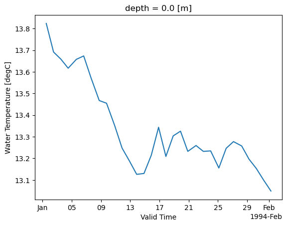
da.hvplot.quadmesh(x='lon', y='lat', geo=True, global_extent=True, tiles='ESRI', cmap='viridis', rasterize=True)

Make a time series

Because the lat/lon is not chunked, we have to read a full slice (117Mb) for each time step. So this is slow and parallelization is limited. But it works.

# slice the time to be once a day, to speed things up
ts = (
    ds["water_temp"]
    .sel(
        depth=0,
        time=slice("1994-01-01", "1994-02-01"),
        lat=slice(40, 50),
        lon=slice(-45, -35),
    )
    .isel(time=slice(None, None, 8))
    .mean(["lat", "lon"])
    .compute()
)

ts.plot()