Introduction to Geospatial Analyses in Python in the Cloud

This is based on the “Examining Environmental Justice through Open Source, Cloud-Native Tools” notebook from Carl Boettiger. Please follow Carl’s notebook for the background. This tutorial just focuses on the code.

Set up

You install a few things that are not on this JHub.

# It is bad to install via pip into a conda environment. I know this
# Remove the commenting and run
# ! pip install odc-stac stac
# ! pip install geopolars

import odc.stac
import rioxarray
from pystac_client import Client
import geopandas as gpd
from rasterstats import zonal_stats 

import dask.distributed
client = dask.distributed.Client()
odc.stac.configure_rio(cloud_defaults=True, client=client)

Data discovery

Here we use a STAC Catalog API to recover a list of candidate data. This example searches for images in a lon-lat bounding box from a collection of Cloud-Optimized-GeoTIFF (COG) images taken by Sentinel2 satellite mission. This function will not download any imagery, it merely gives us a list of metadata about available images.

box = [-122.51, 37.71, -122.36, 37.81]
items = (
  Client.
  open("https://earth-search.aws.element84.com/v1").
  search(
    collections = ['sentinel-2-l2a'],
    bbox = box,
    datetime = "2022-06-01/2022-08-01",
    query={"eo:cloud_cover": {"lt": 20}}).
  item_collection()
)

We pass this list of images to a high-level utilty (gdalcubes) that will do all of the heavy lifting:

subsetting by date
subsetting by bounding box
aggregating by time P1D
reproject into the desired coordinate system
resampling to a desired spatial resolution

data = odc.stac.load(
    items,
    crs="EPSG:4326",
    bands=["nir08", "red"],
    resolution=0.0001,
    bbox=box
)

Calculate NDVI, a widely used measure of greenness that can be used to determine tree cover.

red = data.red
nir = data.nir08

ndvi = (((nir - red) / (red + nir)).
        resample(time="MS").
        median("time", keep_attrs=True).
        compute()
)

# mask out bad pixels
ndvi = ndvi.where(ndvi <= 1)

Plot the result. The long rectangle of Golden Gate Park is clearly visible in the North-West.

import matplotlib as plt
cmap = plt.colormaps.get_cmap('viridis')  # viridis is the default colormap for imshow
cmap.set_bad(color='black')

ndvi.plot.imshow(row="time", cmap=cmap, add_colorbar=False, size=5)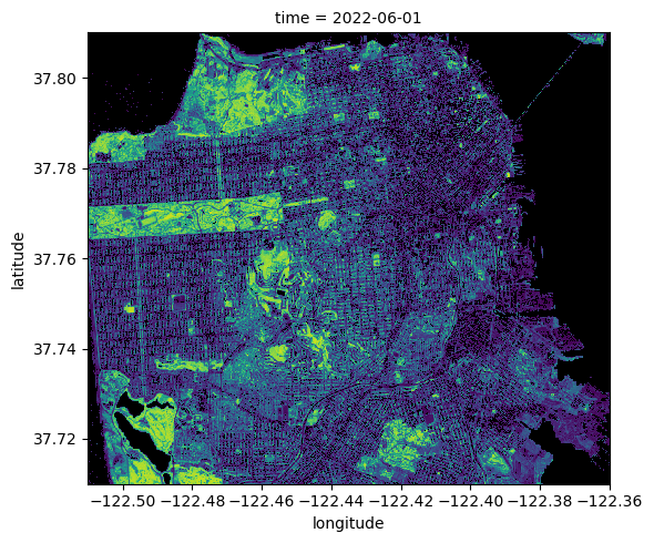

Add the 1937 “red-lining” zones from the Mapping Inequality project. The red-lined zones are spatial vectors.

ndvi.rio.to_raster(raster_path="ndvi.tif", driver="COG")
sf_url = "/vsicurl/https://dsl.richmond.edu/panorama/redlining/static/citiesData/CASanFrancisco1937/geojson.json"
mean_ndvi = zonal_stats(sf_url, "ndvi.tif", stats="mean")

Now we can plot

sf = gpd.read_file(sf_url)
sf["ndvi"] = [x["mean"] for x in mean_ndvi ]
sf.plot(column="ndvi", legend=True)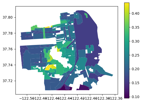

Compute the mean current greenness by 1937 zone.

import geopolars as gpl
import polars as pl

(gpl.
  from_geopandas(sf).
  group_by("grade").
  agg(pl.col("ndvi").mean()).
  sort("grade")
)

shape: (5, 2)

grade	ndvi
str	f64
null	0.157821
"A"	0.338723
"B"	0.247344
"C"	0.231182
"D"	0.225696