Exploring ship echosounder data from the Pacific Hake survey

Jupyter notebook accompanying the manuscript:

Echopype: A Python library for interoperable and scalable processing of ocean sonar data for biological information
Authors: Wu-Jung Lee, Emilio Mayorga, Landung Setiawan, Kavin Nguyen, Imran Majeed, Valentina Staneva

Introduction

Goals

• Illustrate a common workflow for echosounder data conversion, calibration and use. This workflow leverages the standardization applied by echopype and the power, ease of use and familiarity of libraries in the scientific Python ecosystem.
• Extract and visualize data with relative ease using geospatial and temporal filters.

Description

This notebook uses EK60 echosounder data collected during the 2017 Joint U.S.-Canada Integrated Ecosystem and Pacific Hake Acoustic Trawl Survey (‘Pacific Hake Survey’) to illustrate a common workflow for data conversion, calibration and analysis using echopype and core scientific Python software packages, particularly xarray, GeoPandas, pandas and NumPy.

Two days of cloud-hosted .raw data files are accessed by echopype directly from an Amazon Web Services (AWS) S3 “bucket” maintained by the NOAA NCEI Water-Column Sonar Data Archive. The total data used are 170 .raw files at approximately 25 MB each (1 Hz pinging rate from first light to dusk), corresponding to approximately 4.2 GB. With echopype, each file is converted to a standardized representation based on the SONAR-netCDF4 v1.0 convention and saved to the cloud-optimized Zarr format.

Data stored in the netCDF-based SONAR-netCDF4 convention can be conveniently and intuitively manipulated with xarray in combination with related scientific Python packages. Mean Volume Backscattering Strength (MVBS) is computed with echopype from each raw data file and exported to a netCDF file. Here, we define two geographical bounding boxes encompassing two ship tracks and use these to extract corresponding timestamp intervals from the GPS data, and then the corresponding MVBS data based on those intervals. Finally, these extracted MVBS subsets are plotted as track echograms.

Outline

1. Establish AWS S3 file system connection and generate list of target EK60 .raw files
2. Process S3-hosted raw files with echopype: convert, calibrate and export to standardized files
3. Extract and process GPS locations from the Platform group of converted raw files
4. Read MVBS and plot track echograms for time periods corresponding to two ship tracks

Running the notebook

This notebook can be run with a conda environment created using the conda environment file https://github.com/OSOceanAcoustics/echopype-examples/blob/main/binder/environment.yml. The notebook creates two directories, if not already present: ./exports/hakesurvey_convertedzarr and ./exports/hakesurvey_calibratednc. netCDF and Zarr files will be exported there.

Note

We encourage importing echopype as ep for consistency.

from pathlib import Path

import fsspec
import numpy as np
import geopandas as gpd
import xarray as xr

import matplotlib.pyplot as plt
from shapely.geometry import box
import cartopy.crs as ccrs
import cartopy.io.img_tiles as cimgt
from cartopy.mpl.gridliner import LONGITUDE_FORMATTER, LATITUDE_FORMATTER

import echopype as ep
from echopype.qc import exist_reversed_time

import warnings
warnings.simplefilter("ignore", category=DeprecationWarning)

from dask.distributed import Client

client = Client()

client

Client

Client-0457e919-0407-11ef-80d7-820f588673e5

Connection method: Cluster object	Cluster type: distributed.LocalCluster
Dashboard: /user/leewujung/proxy/8787/status

Cluster Info

LocalCluster

5abba2b3

Dashboard: /user/leewujung/proxy/8787/status	Workers: 4
Total threads: 8	Total memory: 31.34 GiB
Status: running	Using processes: True

Scheduler Info

Scheduler

Scheduler-b7dda29b-c5bc-4ea7-ab66-7890b5e5cc79

Comm: tcp://127.0.0.1:38903	Workers: 4
Dashboard: /user/leewujung/proxy/8787/status	Total threads: 8
Started: Just now	Total memory: 31.34 GiB

Workers

Worker: 0

Comm: tcp://127.0.0.1:43205	Total threads: 2
Dashboard: /user/leewujung/proxy/43023/status	Memory: 7.84 GiB
Nanny: tcp://127.0.0.1:40977
Local directory: /tmp/dask-scratch-space/worker-8hk9umex

Worker: 1

Comm: tcp://127.0.0.1:33021	Total threads: 2
Dashboard: /user/leewujung/proxy/33901/status	Memory: 7.84 GiB
Nanny: tcp://127.0.0.1:43227
Local directory: /tmp/dask-scratch-space/worker-rtm3hewa

Worker: 2

Comm: tcp://127.0.0.1:36503	Total threads: 2
Dashboard: /user/leewujung/proxy/34185/status	Memory: 7.84 GiB
Nanny: tcp://127.0.0.1:42299
Local directory: /tmp/dask-scratch-space/worker-sq1_hzly

Worker: 3

Comm: tcp://127.0.0.1:32945	Total threads: 2
Dashboard: /user/leewujung/proxy/38863/status	Memory: 7.84 GiB
Nanny: tcp://127.0.0.1:38595
Local directory: /tmp/dask-scratch-space/worker-ewwsz9bc

Establish AWS S3 file system connection and generate list of target EK60 .raw files

Access and inspect the publicly accessible NCEI WCSD S3 bucket on the AWS cloud as if it were a local file system. This will be done through the Python fsspec file system and bytes storage interface. We will use fsspec.filesystem.glob (fs.glob) to generate a list of all EK60 .raw data files in the bucket, then filter on file names for target dates of interest.

The directory path on the ncei-wcsd-archive S3 bucket is s3://ncei-wcsd-archive/data/raw/Bell_M._Shimada/SH1707/EK60/. All .raw files from the 2017 Hake survey cruise are found here.

fs = fsspec.filesystem('s3', anon=True)

bucket = "ncei-wcsd-archive"
rawdirpath = "data/raw/Bell_M._Shimada/SH1707/EK60"

s3rawfiles = fs.glob(f"{bucket}/{rawdirpath}/*.raw")

# print out the last two S3 raw file paths in the list
s3rawfiles[-2:]

['ncei-wcsd-archive/data/raw/Bell_M._Shimada/SH1707/EK60/Summer2017-D20170913-T180733.raw',
 'ncei-wcsd-archive/data/raw/Bell_M._Shimada/SH1707/EK60/Winter2017-D20170615-T002629.raw']

Generate list of target EK60 .raw files from AWS S3 bucket based on dates. The dates are found in the middle string token (e.g., “D20170913”). Select files from 2 days, 2017-07-28 and 2017-07-29.

s3rawfiles = [
    s3path for s3path in s3rawfiles 
    if any([f"D2017{datestr}" in s3path for datestr in ['0728', '0729']])
]

print(f"There are {len(s3rawfiles)} target raw files available")

There are 170 target raw files available

Process S3-hosted raw files with echopype: convert, calibrate and export to standardized files

Loop through all the selected raw files on S3 and convert, calibrate and generate Mean Volume Backscattering Strength (MVBS). Save the raw converted and MVBS data to local files, as zarr and netCDF, respectively.

def populate_metadata(ed, raw_fname):
    """
    Manually populate into the "ed" EchoData object 
    additional metadata about the dataset and the platform
    """
    
    # -- SONAR-netCDF4 Top-level Group attributes
    survey_name = (
        "2017 Joint U.S.-Canada Integrated Ecosystem and "
        "Pacific Hake Acoustic Trawl Survey ('Pacific Hake Survey')"
    )
    ed['Top-level'].attrs['title'] = f"{survey_name}, file {raw_fname}"
    ed['Top-level'].attrs['summary'] = (
        f"EK60 raw file {raw_fname} from the {survey_name}, converted to a SONAR-netCDF4 file using echopype."
        "Information about the survey program is available at "
        "https://www.fisheries.noaa.gov/west-coast/science-data/"
        "joint-us-canada-integrated-ecosystem-and-pacific-hake-acoustic-trawl-survey"
    )

    # -- SONAR-netCDF4 Platform Group attributes
    # Per SONAR-netCDF4, for platform_type see https://vocab.ices.dk/?ref=311
    ed['Platform'].attrs['platform_type'] = "Research vessel"
    ed['Platform'].attrs['platform_name'] = "Bell M. Shimada"  # A NOAA ship
    ed['Platform'].attrs['platform_code_ICES'] = "315"

Create the directories where the exported files will be saved, if these directories don’t already exist.

base_dpath = Path('./exports/notebook2')
base_dpath.mkdir(exist_ok=True, parents=True)

converted_dpath = Path(base_dpath / 'hakesurvey_convertedzarr')
converted_dpath.mkdir(exist_ok=True)
calibrated_dpath = (base_dpath / 'hakesurvey_calibratednc')
calibrated_dpath.mkdir(exist_ok=True)

echopype processing

EchoData is an echopype object for conveniently handling raw converted data from either raw instrument files or previously converted and standardized raw netCDF4 and Zarr files. It is essentially a container for multiple xarray.Dataset objects, each corresponds to one of the netCDF4 groups specified in the SONAR-netCDF4 convention – the convention followed by echopype. The EchoData object can be used to conveniently accesse and explore the echosounder raw data and for calibration and other processing.

The cell below contains the main echopype workflow steps. For each raw file: - Access file directly from S3 via ep.open_raw to create a converted EchoData object in memory - Add global and platform attributes to EchoData object - Export to a local Zarr dataset (a collection of files encapsulated in a directory) - Generate calibrated Sv and then MVBS from the raw data in the EchoData object - Export MVBS to a local netcdf file

Note: Depending on your internet speed, this cell may take some time to run (potentially 20-30 mins).

# %%time

# for s3rawfpath in s3rawfiles:
#     raw_fpath = Path(s3rawfpath)
#     try:
#         # Access file directly from S3 to create a converted EchoData object in memory
#         ed = ep.open_raw(
#             f"s3://{s3rawfpath}",
#             sonar_model='EK60',
#             storage_options={'anon': True}
#         )
#         # Manually populate additional metadata about the dataset and the platform
#         populate_metadata(ed, raw_fpath.name)

#         # Save to converted Zarr format
#         ed.to_zarr(save_path=converted_dpath, overwrite=True)

#         # Use the EchoData object "ed" to generate calibrated and
#         # computed MVBS files that will be saved to netcdf
#         ds_Sv = ep.calibrate.compute_Sv(ed)
#         ds_MVBS = ep.commongrid.compute_MVBS(
#             ds_Sv,
#             range_meter_bin=5,  # in meters
#             ping_time_bin='20s'  # in seconds
#         )
#         ds_MVBS.to_netcdf(calibrated_dpath / f"MVBS_{raw_fpath.stem}.nc")
#     except Exception as e:
#         print(f"Failed to process raw file {raw_fpath.name}: {e}")

Test for time reversals

Small time reversals are found in EK60 datasets, including the 2017 Pacific Hake survey, where the ping_time (or GPS time1) value may be lower (older) than the preceding ping_time by a second. Such discontinuities can interfere with concatenating individual raw files to produce an aggregated dataset. The capability to identify and address these reversals is in the echopype.qc subpackage.

%%time
for datapath in converted_dpath.glob('*'):
    ed = ep.open_converted(datapath, chunks={})
    # Test for a negative ping_time increment in sequential timestamps, in the Sonar/Beam_group1 group
    if exist_reversed_time(ds=ed['Sonar/Beam_group1'], time_name="ping_time"):
        print(f"Reversed time in {datapath}")

CPU times: user 19.7 s, sys: 6.21 s, total: 25.9 s
Wall time: 2min 9s

There are no time reversals in this two-day dataset, fortunately.

Examine the EchoData object for one of the data files

echopype provides a user-friendly, convenient representation of an EchoData object that leverages the user-friendly xarray Dataset HTML representation. Since an EchoData object is effectively a container for multiple xarray.Dataset objects corresponding to netCDF4 groups, the notebook “print out” provides a summary view of all the groups and interactive access to summaries of each group.

Here, ed is the last object opened in the time reversal test, in the preceding cell.

ed = ep.open_converted(list(converted_dpath.glob('*'))[0], chunks={})

ed

EchoData: standardized raw data from /home/jovyan/shared/echopype-examples/notebooks/exports/notebook2/hakesurvey_convertedzarr/Summer2017-D20170729-T235813.zarr

• Top-level: contains metadata about the SONAR-netCDF4 file format.

  <xarray.Dataset>
  Dimensions:  ()
  Data variables:
      *empty*
  Attributes:
      conventions:                 CF-1.7, SONAR-netCDF4-1.0, ACDD-1.3
      date_created:                2017-07-29T23:58:13Z
      keywords:                    EK60
      processing_level:            Level 1A
      processing_level_url:        https://echopype.readthedocs.io/en/stable/pr...
      sonar_convention_authority:  ICES
      sonar_convention_name:       SONAR-netCDF4
      sonar_convention_version:    1.0
      summary:                     EK60 raw file Summer2017-D20170729-T235813.r...
      title:                       2017 Joint U.S.-Canada Integrated Ecosystem ...

  xarray.Dataset

  • Dimensions:
  • Coordinates: (0)
  • Data variables: (0)
  • Indexes: (0)
  • Attributes: (10)

    conventions :

    CF-1.7, SONAR-netCDF4-1.0, ACDD-1.3

    date_created :

    2017-07-29T23:58:13Z

    keywords :

    EK60

    processing_level :

    Level 1A

    processing_level_url :

    https://echopype.readthedocs.io/en/stable/processing-levels.html

    sonar_convention_authority :

    ICES

    sonar_convention_name :

    SONAR-netCDF4

    sonar_convention_version :

    1.0

    summary :

    EK60 raw file Summer2017-D20170729-T235813.raw from the 2017 Joint U.S.-Canada Integrated Ecosystem and Pacific Hake Acoustic Trawl Survey ('Pacific Hake Survey'), converted to a SONAR-netCDF4 file using echopype.Information about the survey program is available at https://www.fisheries.noaa.gov/west-coast/science-data/joint-us-canada-integrated-ecosystem-and-pacific-hake-acoustic-trawl-survey

    title :

    2017 Joint U.S.-Canada Integrated Ecosystem and Pacific Hake Acoustic Trawl Survey ('Pacific Hake Survey'), file Summer2017-D20170729-T235813.raw

  
  
• Environment: contains information relevant to acoustic propagation through water.

  <xarray.Dataset>
  Dimensions:                 (channel: 3, time1: 534)
  Coordinates:
    * channel                 (channel) <U37 'GPT  18 kHz 009072058c8d 1-1 ES18...
    * time1                   (time1) datetime64[ns] 2017-07-29T23:58:13.128697...
  Data variables:
      absorption_indicative   (channel, time1) float64 dask.array<chunksize=(3, 534), meta=np.ndarray>
      frequency_nominal       (channel) float64 dask.array<chunksize=(3,), meta=np.ndarray>
      sound_speed_indicative  (channel, time1) float64 dask.array<chunksize=(3, 534), meta=np.ndarray>

  xarray.Dataset

  • Dimensions:
    • channel: 3
    • time1: 534
  • Coordinates: (2)
    • channel
      (channel)
      <U37
      'GPT 18 kHz 009072058c8d 1-1 ES...

      long_name :

      Vendor channel ID

      array(['GPT  18 kHz 009072058c8d 1-1 ES18-11',
             'GPT  38 kHz 009072058146 2-1 ES38B',
             'GPT 120 kHz 00907205a6d0 4-1 ES120-7C'], dtype='<U37')

    • time1
      (time1)
      datetime64[ns]
      2017-07-29T23:58:13.128697856 .....

      axis :

      T

      comment :

      Time coordinate corresponding to environmental variables.

      long_name :

      Timestamps for NMEA position datagrams

      standard_name :

      time

      array(['2017-07-29T23:58:13.128697856', '2017-07-29T23:58:15.371826176',
             '2017-07-29T23:58:17.597954048', ..., '2017-07-30T00:17:52.050916864',
             '2017-07-30T00:17:54.266042880', '2017-07-30T00:17:56.492170240'],
            dtype='datetime64[ns]')

  • Data variables: (3)
    • absorption_indicative
      (channel, time1)
      float64
      dask.array<chunksize=(3, 534), meta=np.ndarray>

      long_name :

      Indicative acoustic absorption

      units :

      dB/m

      valid_min :

      0.0

      Array Chunk Bytes 12.52 kiB 12.52 kiB Shape (3, 534) (3, 534) Dask graph 1 chunks in 2 graph layers Data type float64 numpy.ndarray

    • frequency_nominal
      (channel)
      float64
      dask.array<chunksize=(3,), meta=np.ndarray>

      long_name :

      Transducer frequency

      standard_name :

      sound_frequency

      units :

      Hz

      valid_min :

      0.0

      Array Chunk Bytes 24 B 24 B Shape (3,) (3,) Dask graph 1 chunks in 2 graph layers Data type float64 numpy.ndarray

    • sound_speed_indicative
      (channel, time1)
      float64
      dask.array<chunksize=(3, 534), meta=np.ndarray>

      long_name :

      Indicative sound speed

      standard_name :

      speed_of_sound_in_sea_water

      units :

      m/s

      valid_min :

      0.0

      Array Chunk Bytes 12.52 kiB 12.52 kiB Shape (3, 534) (3, 534) Dask graph 1 chunks in 2 graph layers Data type float64 numpy.ndarray

  • Indexes: (2)
    • channel
      PandasIndex

      PandasIndex(Index(['GPT  18 kHz 009072058c8d 1-1 ES18-11',
             'GPT  38 kHz 009072058146 2-1 ES38B',
             'GPT 120 kHz 00907205a6d0 4-1 ES120-7C'],
            dtype='object', name='channel'))

    • time1
      PandasIndex

      PandasIndex(DatetimeIndex(['2017-07-29 23:58:13.128697856',
                     '2017-07-29 23:58:15.371826176',
                     '2017-07-29 23:58:17.597954048',
                     '2017-07-29 23:58:19.813082112',
                        '2017-07-29 23:58:22.038208',
                     '2017-07-29 23:58:24.254332928',
                     '2017-07-29 23:58:26.470460928',
                     '2017-07-29 23:58:28.696588800',
                     '2017-07-29 23:58:30.912715776',
                     '2017-07-29 23:58:33.138844160',
                     ...
                     '2017-07-30 00:17:36.490025984',
                     '2017-07-30 00:17:38.716151808',
                     '2017-07-30 00:17:40.951281152',
                     '2017-07-30 00:17:43.178409984',
                        '2017-07-30 00:17:45.393536',
                     '2017-07-30 00:17:47.619662848',
                     '2017-07-30 00:17:49.835790848',
                     '2017-07-30 00:17:52.050916864',
                     '2017-07-30 00:17:54.266042880',
                     '2017-07-30 00:17:56.492170240'],
                    dtype='datetime64[ns]', name='time1', length=534, freq=None))

  • Attributes: (0)

  
  
• Platform: contains information about the platform on which the sonar is installed.

  <xarray.Dataset>
  Dimensions:              (channel: 3, time1: 1676, time2: 534)
  Coordinates:
    * channel              (channel) <U37 'GPT  18 kHz 009072058c8d 1-1 ES18-11...
    * time1                (time1) datetime64[ns] 2017-07-29T23:58:13.511395840...
    * time2                (time2) datetime64[ns] 2017-07-29T23:58:13.128697856...
  Data variables: (12/20)
      MRU_offset_x         float64 ...
      MRU_offset_y         float64 ...
      MRU_offset_z         float64 ...
      MRU_rotation_x       float64 ...
      MRU_rotation_y       float64 ...
      MRU_rotation_z       float64 ...
      ...                   ...
      sentence_type        (time1) <U3 dask.array<chunksize=(1676,), meta=np.ndarray>
      transducer_offset_x  (channel) float64 dask.array<chunksize=(3,), meta=np.ndarray>
      transducer_offset_y  (channel) float64 dask.array<chunksize=(3,), meta=np.ndarray>
      transducer_offset_z  (channel) float64 dask.array<chunksize=(3,), meta=np.ndarray>
      vertical_offset      (time2) float64 dask.array<chunksize=(534,), meta=np.ndarray>
      water_level          float64 ...
  Attributes:
      platform_code_ICES:  315
      platform_name:       Bell M. Shimada
      platform_type:       Research vessel

  xarray.Dataset

  • Dimensions:
    • channel: 3
    • time1: 1676
    • time2: 534
  • Coordinates: (3)
    • channel
      (channel)
      <U37
      'GPT 18 kHz 009072058c8d 1-1 ES...

      long_name :

      Vendor channel ID

      array(['GPT  18 kHz 009072058c8d 1-1 ES18-11',
             'GPT  38 kHz 009072058146 2-1 ES38B',
             'GPT 120 kHz 00907205a6d0 4-1 ES120-7C'], dtype='<U37')

    • time1
      (time1)
      datetime64[ns]
      2017-07-29T23:58:13.511395840 .....

      axis :

      T

      comment :

      Time coordinate corresponding to NMEA position data.

      long_name :

      Timestamps for NMEA datagrams

      standard_name :

      time

      array(['2017-07-29T23:58:13.511395840', '2017-07-29T23:58:13.669727232',
             '2017-07-29T23:58:13.948889088', ..., '2017-07-30T00:17:57.274190848',
             '2017-07-30T00:17:59.223481856', '2017-07-30T00:17:59.381813248'],
            dtype='datetime64[ns]')

    • time2
      (time2)
      datetime64[ns]
      2017-07-29T23:58:13.128697856 .....

      axis :

      T

      comment :

      Time coordinate corresponding to platform motion and orientation data.

      long_name :

      Timestamps for platform motion and orientation data

      standard_name :

      time

      array(['2017-07-29T23:58:13.128697856', '2017-07-29T23:58:15.371826176',
             '2017-07-29T23:58:17.597954048', ..., '2017-07-30T00:17:52.050916864',
             '2017-07-30T00:17:54.266042880', '2017-07-30T00:17:56.492170240'],
            dtype='datetime64[ns]')

  • Data variables: (20)
    • MRU_offset_x
      ()
      float64
      ...

      long_name :

      Distance along the x-axis from the platform coordinate system origin to the motion reference unit sensor origin

      units :

      m

      [1 values with dtype=float64]

    • MRU_offset_y
      ()
      float64
      ...

      long_name :

      Distance along the y-axis from the platform coordinate system origin to the motion reference unit sensor origin

      units :

      m

      [1 values with dtype=float64]

    • MRU_offset_z
      ()
      float64
      ...

      long_name :

      Distance along the z-axis from the platform coordinate system origin to the motion reference unit sensor origin

      units :

      m

      [1 values with dtype=float64]

    • MRU_rotation_x
      ()
      float64
      ...

      long_name :

      Extrinsic rotation about the x-axis from the platform to MRU coordinate systems

      units :

      arc_degree

      valid_range :

      (–180.0, 180.0)

      [1 values with dtype=float64]

    • MRU_rotation_y
      ()
      float64
      ...

      long_name :

      Extrinsic rotation about the y-axis from the platform to MRU coordinate systems

      units :

      arc_degree

      valid_range :

      (–180.0, 180.0)

      [1 values with dtype=float64]

    • MRU_rotation_z
      ()
      float64
      ...

      long_name :

      Extrinsic rotation about the z-axis from the platform to MRU coordinate systems

      units :

      arc_degree

      valid_range :

      (–180.0, 180.0)

      [1 values with dtype=float64]

    • frequency_nominal
      (channel)
      float64
      dask.array<chunksize=(3,), meta=np.ndarray>

      long_name :

      Transducer frequency

      standard_name :

      sound_frequency

      units :

      Hz

      valid_min :

      0.0

      Array Chunk Bytes 24 B 24 B Shape (3,) (3,) Dask graph 1 chunks in 2 graph layers Data type float64 numpy.ndarray

    • latitude
      (time1)
      float64
      dask.array<chunksize=(1676,), meta=np.ndarray>

      long_name :

      Platform latitude

      standard_name :

      latitude

      units :

      degrees_north

      valid_range :

      (-90.0, 90.0)

      Array Chunk Bytes 13.09 kiB 13.09 kiB Shape (1676,) (1676,) Dask graph 1 chunks in 2 graph layers Data type float64 numpy.ndarray

    • longitude
      (time1)
      float64
      dask.array<chunksize=(1676,), meta=np.ndarray>

      long_name :

      Platform longitude

      standard_name :

      longitude

      units :

      degrees_east

      valid_range :

      (-180.0, 180.0)

      Array Chunk Bytes 13.09 kiB 13.09 kiB Shape (1676,) (1676,) Dask graph 1 chunks in 2 graph layers Data type float64 numpy.ndarray

    • pitch
      (time2)
      float64
      dask.array<chunksize=(534,), meta=np.ndarray>

      long_name :

      Platform pitch

      standard_name :

      platform_pitch_angle

      units :

      arc_degree

      valid_range :

      (-90.0, 90.0)

      Array Chunk Bytes 4.17 kiB 4.17 kiB Shape (534,) (534,) Dask graph 1 chunks in 2 graph layers Data type float64 numpy.ndarray

    • position_offset_x
      ()
      float64
      ...

      long_name :

      Distance along the x-axis from the platform coordinate system origin to the latitude/longitude sensor origin

      units :

      m

      [1 values with dtype=float64]

    • position_offset_y
      ()
      float64
      ...

      long_name :

      Distance along the y-axis from the platform coordinate system origin to the latitude/longitude sensor origin

      units :

      m

      [1 values with dtype=float64]

    • position_offset_z
      ()
      float64
      ...

      long_name :

      Distance along the z-axis from the platform coordinate system origin to the latitude/longitude sensor origin

      units :

      m

      [1 values with dtype=float64]

    • roll
      (time2)
      float64
      dask.array<chunksize=(534,), meta=np.ndarray>

      long_name :

      Platform roll

      standard_name :

      platform_roll_angle

      units :

      arc_degree

      valid_range :

      (-90.0, 90.0)

      Array Chunk Bytes 4.17 kiB 4.17 kiB Shape (534,) (534,) Dask graph 1 chunks in 2 graph layers Data type float64 numpy.ndarray

    • transducer_offset_x
      (channel)
      float64
      dask.array<chunksize=(3,), meta=np.ndarray>

      long_name :

      x-axis distance from the platform coordinate system origin to the sonar transducer

      units :

      m

      Array Chunk Bytes 24 B 24 B Shape (3,) (3,) Dask graph 1 chunks in 2 graph layers Data type float64 numpy.ndarray

    • transducer_offset_y
      (channel)
      float64
      dask.array<chunksize=(3,), meta=np.ndarray>

      long_name :

      y-axis distance from the platform coordinate system origin to the sonar transducer

      units :

      m

      Array Chunk Bytes 24 B 24 B Shape (3,) (3,) Dask graph 1 chunks in 2 graph layers Data type float64 numpy.ndarray

    • transducer_offset_z
      (channel)
      float64
      dask.array<chunksize=(3,), meta=np.ndarray>

      long_name :

      z-axis distance from the platform coordinate system origin to the sonar transducer

      units :

      m

      Array Chunk Bytes 24 B 24 B Shape (3,) (3,) Dask graph 1 chunks in 2 graph layers Data type float64 numpy.ndarray

    • vertical_offset
      (time2)
      float64
      dask.array<chunksize=(534,), meta=np.ndarray>

      long_name :

      Platform vertical offset from nominal water level

      units :

      m

      Array Chunk Bytes 4.17 kiB 4.17 kiB Shape (534,) (534,) Dask graph 1 chunks in 2 graph layers Data type float64 numpy.ndarray

  • Indexes: (1)
    • beam_group
      PandasIndex

      PandasIndex(Index(['Beam_group1'], dtype='object', name='beam_group'))

  • Attributes: (6)

    sonar_manufacturer :

    Simrad

    sonar_model :

    EK60

    sonar_serial_number :

    sonar_software_name :

    ER60

    sonar_software_version :

    2.4.3

    sonar_type :

    echosounder

  
  
• Beam_group1: contains backscatter power (uncalibrated) and other beam or channel-specific data, including split-beam angle data when they exist.

  <xarray.Dataset>
  Dimensions:                        (channel: 3, ping_time: 534,
                                      range_sample: 3957)
  Coordinates:
    * channel                        (channel) <U37 'GPT  18 kHz 009072058c8d 1...
    * ping_time                      (ping_time) datetime64[ns] 2017-07-29T23:5...
    * range_sample                   (range_sample) int64 0 1 2 ... 3954 3955 3956
  Data variables: (12/29)
      angle_alongship                (channel, ping_time, range_sample) float32 dask.array<chunksize=(3, 534, 3957), meta=np.ndarray>
      angle_athwartship              (channel, ping_time, range_sample) float32 dask.array<chunksize=(3, 534, 3957), meta=np.ndarray>
      angle_offset_alongship         (channel) float64 dask.array<chunksize=(3,), meta=np.ndarray>
      angle_offset_athwartship       (channel) float64 dask.array<chunksize=(3,), meta=np.ndarray>
      angle_sensitivity_alongship    (channel) float64 dask.array<chunksize=(3,), meta=np.ndarray>
      angle_sensitivity_athwartship  (channel) float64 dask.array<chunksize=(3,), meta=np.ndarray>
      ...                             ...
      transmit_bandwidth             (channel, ping_time) float64 dask.array<chunksize=(3, 534), meta=np.ndarray>
      transmit_duration_nominal      (channel, ping_time) float64 dask.array<chunksize=(3, 534), meta=np.ndarray>
      transmit_frequency_start       (channel) float64 dask.array<chunksize=(3,), meta=np.ndarray>
      transmit_frequency_stop        (channel) float64 dask.array<chunksize=(3,), meta=np.ndarray>
      transmit_power                 (channel, ping_time) float64 dask.array<chunksize=(3, 534), meta=np.ndarray>
      transmit_type                  <U2 ...
  Attributes:
      beam_mode:              vertical
      conversion_equation_t:  type_3

  xarray.Dataset

  • Dimensions:
    • channel: 3
    • ping_time: 534
    • range_sample: 3957
  • Coordinates: (3)
    • channel
      (channel)
      <U37
      'GPT 18 kHz 009072058c8d 1-1 ES...

      long_name :

      Vendor channel ID

      array(['GPT  18 kHz 009072058c8d 1-1 ES18-11',
             'GPT  38 kHz 009072058146 2-1 ES38B',
             'GPT 120 kHz 00907205a6d0 4-1 ES120-7C'], dtype='<U37')

    • ping_time
      (ping_time)
      datetime64[ns]
      2017-07-29T23:58:13.128697856 .....

      axis :

      T

      long_name :

      Timestamp of each ping

      standard_name :

      time

      array(['2017-07-29T23:58:13.128697856', '2017-07-29T23:58:15.371826176',
             '2017-07-29T23:58:17.597954048', ..., '2017-07-30T00:17:52.050916864',
             '2017-07-30T00:17:54.266042880', '2017-07-30T00:17:56.492170240'],
            dtype='datetime64[ns]')

    • range_sample
      (range_sample)
      int64
      0 1 2 3 4 ... 3953 3954 3955 3956

      long_name :

      Along-range sample number, base 0

      array([   0,    1,    2, ..., 3954, 3955, 3956])

  • Data variables: (29)
    • angle_alongship
      (channel, ping_time, range_sample)
      float32
      dask.array<chunksize=(3, 534, 3957), meta=np.ndarray>

      comment :

      Introduced in echopype for Simrad echosounders. The alongship angle corresponds to the minor angle in SONAR-netCDF4 vers 2.

      long_name :

      electrical alongship angle

      Array Chunk Bytes 24.18 MiB 24.18 MiB Shape (3, 534, 3957) (3, 534, 3957) Dask graph 1 chunks in 2 graph layers Data type float32 numpy.ndarray

    • angle_athwartship
      (channel, ping_time, range_sample)
      float32
      dask.array<chunksize=(3, 534, 3957), meta=np.ndarray>

      comment :

      Introduced in echopype for Simrad echosounders. The athwartship angle corresponds to the major angle in SONAR-netCDF4 vers 2.

      long_name :

      electrical athwartship angle

      Array Chunk Bytes 24.18 MiB 24.18 MiB Shape (3, 534, 3957) (3, 534, 3957) Dask graph 1 chunks in 2 graph layers Data type float32 numpy.ndarray

    • angle_offset_alongship
      (channel)
      float64
      dask.array<chunksize=(3,), meta=np.ndarray>

      comment :

      Introduced in echopype for Simrad echosounders. The alongship angle corresponds to the minor angle in SONAR-netCDF4 vers 2.

      long_name :

      electrical alongship angle offset of the transducer

      Array Chunk Bytes 24 B 24 B Shape (3,) (3,) Dask graph 1 chunks in 2 graph layers Data type float64 numpy.ndarray

    • angle_offset_athwartship
      (channel)
      float64
      dask.array<chunksize=(3,), meta=np.ndarray>

      comment :

      Introduced in echopype for Simrad echosounders. The athwartship angle corresponds to the major angle in SONAR-netCDF4 vers 2.

      long_name :

      electrical athwartship angle offset of the transducer

      Array Chunk Bytes 24 B 24 B Shape (3,) (3,) Dask graph 1 chunks in 2 graph layers Data type float64 numpy.ndarray

    • angle_sensitivity_alongship
      (channel)
      float64
      dask.array<chunksize=(3,), meta=np.ndarray>

      comment :

      Introduced in echopype for Simrad echosounders. The alongship angle corresponds to the minor angle in SONAR-netCDF4 vers 2.

      long_name :

      alongship angle sensitivity of the transducer

      Array Chunk Bytes 24 B 24 B Shape (3,) (3,) Dask graph 1 chunks in 2 graph layers Data type float64 numpy.ndarray

    • angle_sensitivity_athwartship
      (channel)
      float64
      dask.array<chunksize=(3,), meta=np.ndarray>

      comment :

      Introduced in echopype for Simrad echosounders. The athwartship angle corresponds to the major angle in SONAR-netCDF4 vers 2.

      long_name :

      athwartship angle sensitivity of the transducer

      Array Chunk Bytes 24 B 24 B Shape (3,) (3,) Dask graph 1 chunks in 2 graph layers Data type float64 numpy.ndarray

    • backscatter_r
      (channel, ping_time, range_sample)
      float32
      dask.array<chunksize=(3, 534, 3957), meta=np.ndarray>

      long_name :

      Raw backscatter measurements (real part)

      units :

      dB

      Array Chunk Bytes 24.18 MiB 24.18 MiB Shape (3, 534, 3957) (3, 534, 3957) Dask graph 1 chunks in 2 graph layers Data type float32 numpy.ndarray

    • beam_direction_x
      (channel)
      float64
      dask.array<chunksize=(3,), meta=np.ndarray>

      long_name :

      x-component of the vector that gives the pointing direction of the beam, in sonar beam coordinate system

      units :

      1

      valid_range :

      [-1.0, 1.0]

      Array Chunk Bytes 24 B 24 B Shape (3,) (3,) Dask graph 1 chunks in 2 graph layers Data type float64 numpy.ndarray

    • beam_direction_y
      (channel)
      float64
      dask.array<chunksize=(3,), meta=np.ndarray>

      long_name :

      y-component of the vector that gives the pointing direction of the beam, in sonar beam coordinate system

      units :

      1

      valid_range :

      [-1.0, 1.0]

      Array Chunk Bytes 24 B 24 B Shape (3,) (3,) Dask graph 1 chunks in 2 graph layers Data type float64 numpy.ndarray

    • beam_direction_z
      (channel)
      float64
      dask.array<chunksize=(3,), meta=np.ndarray>

      long_name :

      z-component of the vector that gives the pointing direction of the beam, in sonar beam coordinate system

      units :

      1

      valid_range :

      [-1.0, 1.0]

      Array Chunk Bytes 24 B 24 B Shape (3,) (3,) Dask graph 1 chunks in 2 graph layers Data type float64 numpy.ndarray

    • beam_stabilisation
      ()
      int8
      ...

      flag_meanings :

      ['not stabilised', 'stabilised']

      flag_values :

      [0, 1]

      long_name :

      Beam stabilisation applied (or not)

      [1 values with dtype=int8]

    • beam_type
      (channel)
      int64
      dask.array<chunksize=(3,), meta=np.ndarray>

      long_name :

      type of transducer (0-single, 1-split)

      Array Chunk Bytes 24 B 24 B Shape (3,) (3,) Dask graph 1 chunks in 2 graph layers Data type int64 numpy.ndarray

    • beamwidth_twoway_alongship
      (channel)
      float64
      dask.array<chunksize=(3,), meta=np.ndarray>

      comment :

      Introduced in echopype for Simrad echosounders to avoid potential confusion with convention definitions. The alongship angle corresponds to the minor angle in SONAR-netCDF4 vers 2. The convention defines one-way transmit or receive beamwidth (beamwidth_receive_minor and beamwidth_transmit_minor), but Simrad echosounders record two-way beamwidth in the data.

      long_name :

      Half power two-way beam width along alongship axis of beam

      units :

      arc_degree

      valid_range :

      [0.0, 360.0]

      Array Chunk Bytes 24 B 24 B Shape (3,) (3,) Dask graph 1 chunks in 2 graph layers Data type float64 numpy.ndarray

    • beamwidth_twoway_athwartship
      (channel)
      float64
      dask.array<chunksize=(3,), meta=np.ndarray>

      comment :

      Introduced in echopype for Simrad echosounders to avoid potential confusion with convention definitions. The athwartship angle corresponds to the major angle in SONAR-netCDF4 vers 2. The convention defines one-way transmit or receive beamwidth (beamwidth_receive_major and beamwidth_transmit_major), but Simrad echosounders record two-way beamwidth in the data.

      long_name :

      Half power two-way beam width along athwartship axis of beam

      units :

      arc_degree

      valid_range :

      [0.0, 360.0]

      Array Chunk Bytes 24 B 24 B Shape (3,) (3,) Dask graph 1 chunks in 2 graph layers Data type float64 numpy.ndarray

    • channel_mode
      (channel, ping_time)
      int8
      dask.array<chunksize=(3, 534), meta=np.ndarray>

      comment :

      From transmit_mode in the EK60 datagram

      flag_meanings :

      ['Unknown', 'Active', 'Passive', 'Test']

      flag_values :

      [-1, 0, 1, 2]

      long_name :

      Transceiver mode

      Array Chunk Bytes 1.56 kiB 1.56 kiB Shape (3, 534) (3, 534) Dask graph 1 chunks in 2 graph layers Data type int8 numpy.ndarray

    • data_type
      (channel, ping_time)
      float32
      dask.array<chunksize=(3, 534), meta=np.ndarray>

      flag_meanings :

      ['power only', 'angle only', 'power and angle']

      flag_values :

      [1, 2, 3]

      long_name :

      recorded data type (1=power only, 2=angle only, 3=power and angle)

      Array Chunk Bytes 6.26 kiB 6.26 kiB Shape (3, 534) (3, 534) Dask graph 1 chunks in 2 graph layers Data type float32 numpy.ndarray

    • equivalent_beam_angle
      (channel)
      float64
      dask.array<chunksize=(3,), meta=np.ndarray>

      long_name :

      Equivalent beam angle

      units :

      sr

      valid_range :

      [0.0, 12.566370614359172]

      Array Chunk Bytes 24 B 24 B Shape (3,) (3,) Dask graph 1 chunks in 2 graph layers Data type float64 numpy.ndarray

    • frequency_nominal
      (channel)
      float64
      dask.array<chunksize=(3,), meta=np.ndarray>

      long_name :

      Transducer frequency

      standard_name :

      sound_frequency

      units :

      Hz

      valid_min :

      0.0

      Array Chunk Bytes 24 B 24 B Shape (3,) (3,) Dask graph 1 chunks in 2 graph layers Data type float64 numpy.ndarray

    • gain_correction
      (channel)
      float64
      dask.array<chunksize=(3,), meta=np.ndarray>

      long_name :

      Gain correction

      units :

      dB

      Array Chunk Bytes 24 B 24 B Shape (3,) (3,) Dask graph 1 chunks in 2 graph layers Data type float64 numpy.ndarray

    • non_quantitative_processing
      ()
      int16
      ...

      flag_meanings :

      ['None']

      flag_values :

      [0]

      long_name :

      Presence or not of non-quantitative processing applied to the backscattering data (sonar specific)

      [1 values with dtype=int16]

    • sample_interval
      (channel, ping_time)
      float64
      dask.array<chunksize=(3, 534), meta=np.ndarray>

      long_name :

      Interval between recorded raw data samples

      units :

      s

      valid_min :

      0.0

      Array Chunk Bytes 12.52 kiB 12.52 kiB Shape (3, 534) (3, 534) Dask graph 1 chunks in 2 graph layers Data type float64 numpy.ndarray

    • sample_time_offset
      (channel, ping_time)
      float64
      dask.array<chunksize=(3, 534), meta=np.ndarray>

      long_name :

      Time offset that is subtracted from the timestamp of each sample

      units :

      s

      Array Chunk Bytes 12.52 kiB 12.52 kiB Shape (3, 534) (3, 534) Dask graph 1 chunks in 2 graph layers Data type float64 numpy.ndarray

    • transmit_bandwidth
      (channel, ping_time)
      float64
      dask.array<chunksize=(3, 534), meta=np.ndarray>

      long_name :

      Nominal bandwidth of transmitted pulse

      units :

      Hz

      valid_min :

      0.0

      Array Chunk Bytes 12.52 kiB 12.52 kiB Shape (3, 534) (3, 534) Dask graph 1 chunks in 2 graph layers Data type float64 numpy.ndarray

    • transmit_duration_nominal
      (channel, ping_time)
      float64
      dask.array<chunksize=(3, 534), meta=np.ndarray>

      long_name :

      Nominal bandwidth of transmitted pulse

      units :

      s

      valid_min :

      0.0

      Array Chunk Bytes 12.52 kiB 12.52 kiB Shape (3, 534) (3, 534) Dask graph 1 chunks in 2 graph layers Data type float64 numpy.ndarray

    • transmit_frequency_start
      (channel)
      float64
      dask.array<chunksize=(3,), meta=np.ndarray>

      long_name :

      Start frequency in transmitted pulse

      standard_name :

      sound_frequency

      units :

      Hz

      valid_min :

      0.0

      Array Chunk Bytes 24 B 24 B Shape (3,) (3,) Dask graph 1 chunks in 2 graph layers Data type float64 numpy.ndarray

    • transmit_frequency_stop
      (channel)
      float64
      dask.array<chunksize=(3,), meta=np.ndarray>

      long_name :

      Stop frequency in transmitted pulse

      standard_name :

      sound_frequency

      units :

      Hz

      valid_min :

      0.0

      Array Chunk Bytes 24 B 24 B Shape (3,) (3,) Dask graph 1 chunks in 2 graph layers Data type float64 numpy.ndarray

    • transmit_power
      (channel, ping_time)
      float64
      dask.array<chunksize=(3, 534), meta=np.ndarray>

      long_name :

      Nominal transmit power

      units :

      W

      valid_min :

      0.0

      Array Chunk Bytes 12.52 kiB 12.52 kiB Shape (3, 534) (3, 534) Dask graph 1 chunks in 2 graph layers Data type float64 numpy.ndarray

    • transmit_type
      ()
      <U2
      ...

      flag_meanings :

      ['Continuous Wave – a pulse nominally of one frequency']

      flag_values :

      ['CW']

      long_name :

      Type of transmitted pulse

      [1 values with dtype=<U2]

  • Indexes: (3)
    • channel
      PandasIndex

      PandasIndex(Index(['GPT  18 kHz 009072058c8d 1-1 ES18-11',
             'GPT  38 kHz 009072058146 2-1 ES38B',
             'GPT 120 kHz 00907205a6d0 4-1 ES120-7C'],
            dtype='object', name='channel'))

    • ping_time
      PandasIndex

      PandasIndex(DatetimeIndex(['2017-07-29 23:58:13.128697856',
                     '2017-07-29 23:58:15.371826176',
                     '2017-07-29 23:58:17.597954048',
                     '2017-07-29 23:58:19.813082112',
                        '2017-07-29 23:58:22.038208',
                     '2017-07-29 23:58:24.254332928',
                     '2017-07-29 23:58:26.470460928',
                     '2017-07-29 23:58:28.696588800',
                     '2017-07-29 23:58:30.912715776',
                     '2017-07-29 23:58:33.138844160',
                     ...
                     '2017-07-30 00:17:36.490025984',
                     '2017-07-30 00:17:38.716151808',
                     '2017-07-30 00:17:40.951281152',
                     '2017-07-30 00:17:43.178409984',
                        '2017-07-30 00:17:45.393536',
                     '2017-07-30 00:17:47.619662848',
                     '2017-07-30 00:17:49.835790848',
                     '2017-07-30 00:17:52.050916864',
                     '2017-07-30 00:17:54.266042880',
                     '2017-07-30 00:17:56.492170240'],
                    dtype='datetime64[ns]', name='ping_time', length=534, freq=None))

    • range_sample
      PandasIndex

      PandasIndex(Int64Index([   0,    1,    2,    3,    4,    5,    6,    7,    8,    9,
                  ...
                  3947, 3948, 3949, 3950, 3951, 3952, 3953, 3954, 3955, 3956],
                 dtype='int64', name='range_sample', length=3957))

  • Attributes: (2)

    beam_mode :

    vertical

    conversion_equation_t :

    type_3

  
  
• Vendor_specific: contains vendor-specific information about the sonar and the data.

  <xarray.Dataset>
  Dimensions:            (channel: 3, pulse_length_bin: 5)
  Coordinates:
    * channel            (channel) <U37 'GPT  18 kHz 009072058c8d 1-1 ES18-11' ...
    * pulse_length_bin   (pulse_length_bin) int64 0 1 2 3 4
  Data variables:
      frequency_nominal  (channel) float64 dask.array<chunksize=(3,), meta=np.ndarray>
      gain_correction    (channel, pulse_length_bin) float64 dask.array<chunksize=(3, 5), meta=np.ndarray>
      pulse_length       (channel, pulse_length_bin) float64 dask.array<chunksize=(3, 5), meta=np.ndarray>
      sa_correction      (channel, pulse_length_bin) float64 dask.array<chunksize=(3, 5), meta=np.ndarray>

  xarray.Dataset

  • Dimensions:
    • channel: 3
    • pulse_length_bin: 5
  • Coordinates: (2)
    • channel
      (channel)
      <U37
      'GPT 18 kHz 009072058c8d 1-1 ES...

      long_name :

      Vendor channel ID

      array(['GPT  18 kHz 009072058c8d 1-1 ES18-11',
             'GPT  38 kHz 009072058146 2-1 ES38B',
             'GPT 120 kHz 00907205a6d0 4-1 ES120-7C'], dtype='<U37')

    • pulse_length_bin
      (pulse_length_bin)
      int64
      0 1 2 3 4

      array([0, 1, 2, 3, 4])

  • Data variables: (4)
    • frequency_nominal
      (channel)
      float64
      dask.array<chunksize=(3,), meta=np.ndarray>

      long_name :

      Transducer frequency

      standard_name :

      sound_frequency

      units :

      Hz

      valid_min :

      0.0

      Array Chunk Bytes 24 B 24 B Shape (3,) (3,) Dask graph 1 chunks in 2 graph layers Data type float64 numpy.ndarray

    • gain_correction
      (channel, pulse_length_bin)
      float64
      dask.array<chunksize=(3, 5), meta=np.ndarray>

      Array Chunk Bytes 120 B 120 B Shape (3, 5) (3, 5) Dask graph 1 chunks in 2 graph layers Data type float64 numpy.ndarray

    • pulse_length
      (channel, pulse_length_bin)
      float64
      dask.array<chunksize=(3, 5), meta=np.ndarray>

      Array Chunk Bytes 120 B 120 B Shape (3, 5) (3, 5) Dask graph 1 chunks in 2 graph layers Data type float64 numpy.ndarray

    • sa_correction
      (channel, pulse_length_bin)
      float64
      dask.array<chunksize=(3, 5), meta=np.ndarray>

      Array Chunk Bytes 120 B 120 B Shape (3, 5) (3, 5) Dask graph 1 chunks in 2 graph layers Data type float64 numpy.ndarray

  • Indexes: (2)
    • channel
      PandasIndex

      PandasIndex(Index(['GPT  18 kHz 009072058c8d 1-1 ES18-11',
             'GPT  38 kHz 009072058146 2-1 ES38B',
             'GPT 120 kHz 00907205a6d0 4-1 ES120-7C'],
            dtype='object', name='channel'))

    • pulse_length_bin
      PandasIndex

      PandasIndex(Int64Index([0, 1, 2, 3, 4], dtype='int64', name='pulse_length_bin'))

  • Attributes: (0)

  
  

Extract and process GPS locations from the Platform group of converted raw files

Use xarray.open_mfdataset to open the Platform group from all the converted raw netcdf files as a single concatenated (combined) xarray dataset. Then extract GPS time1 (time stamp), latitude and longitude from this group and transform that data into a GeoPandas GeoDataFrame containing point-geometry objects that are readily manipulated via geospatial operations. A GeoDataFrame adds geospatial capabilities to a Pandas DataFrame.

Due to the presence of multiple time coordinates in this group, care must be taken in defining how the concatenation (combine) operation is to be performed. This is captured in the arguments passed to open_mfdataset.

%%time
platform_ds = xr.open_mfdataset(
    str(converted_dpath / '*.zarr'), group='Platform', 
    engine='zarr',
    data_vars='minimal', coords='minimal',
    combine='nested', chunks={}
)

CPU times: user 1min 52s, sys: 12.3 s, total: 2min 5s
Wall time: 3min 34s

platform_ds

<xarray.Dataset>
Dimensions:              (channel: 3, time1: 244846, time2: 88959)
Coordinates:
  * channel              (channel) <U37 'GPT  18 kHz 009072058c8d 1-1 ES18-11...
  * time1                (time1) datetime64[ns] 2017-07-28T00:05:36.103314944...
  * time2                (time2) datetime64[ns] 2017-07-28T00:05:34.897271808...
Data variables: (12/20)
    MRU_offset_x         float64 nan
    MRU_offset_y         float64 nan
    MRU_offset_z         float64 nan
    MRU_rotation_x       float64 nan
    MRU_rotation_y       float64 nan
    MRU_rotation_z       float64 nan
    ...                   ...
    sentence_type        (time1) object dask.array<chunksize=(244846,), meta=np.ndarray>
    transducer_offset_x  (channel) float64 dask.array<chunksize=(3,), meta=np.ndarray>
    transducer_offset_y  (channel) float64 dask.array<chunksize=(3,), meta=np.ndarray>
    transducer_offset_z  (channel) float64 dask.array<chunksize=(3,), meta=np.ndarray>
    vertical_offset      (time2) float64 dask.array<chunksize=(88959,), meta=np.ndarray>
    water_level          float64 9.15
Attributes:
    platform_code_ICES:  315
    platform_name:       Bell M. Shimada
    platform_type:       Research vessel

xarray.Dataset

• Dimensions:
  • channel: 3
  • time1: 244846
  • time2: 88959
• Coordinates: (3)
  • channel
    (channel)
    <U37
    'GPT 18 kHz 009072058c8d 1-1 ES...

    long_name :

    Vendor channel ID

    array(['GPT  18 kHz 009072058c8d 1-1 ES18-11',
           'GPT  38 kHz 009072058146 2-1 ES38B',
           'GPT 120 kHz 00907205a6d0 4-1 ES120-7C'], dtype='<U37')

  • time1
    (time1)
    datetime64[ns]
    2017-07-28T00:05:36.103314944 .....

    axis :

    T

    comment :

    Time coordinate corresponding to NMEA position data.

    long_name :

    Timestamps for NMEA datagrams

    standard_name :

    time

    array(['2017-07-28T00:05:36.103314944', '2017-07-28T00:05:37.511096832',
           '2017-07-28T00:05:37.669428224', ..., '2017-07-30T00:17:57.274190848',
           '2017-07-30T00:17:59.223481856', '2017-07-30T00:17:59.381813248'],
          dtype='datetime64[ns]')

  • time2
    (time2)
    datetime64[ns]
    2017-07-28T00:05:34.897271808 .....

    axis :

    T

    comment :

    Time coordinate corresponding to platform motion and orientation data.

    long_name :

    Timestamps for platform motion and orientation data

    standard_name :

    time

    array(['2017-07-28T00:05:34.897271808', '2017-07-28T00:05:37.162400768',
           '2017-07-28T00:05:38.404471808', ..., '2017-07-30T00:17:52.050916864',
           '2017-07-30T00:17:54.266042880', '2017-07-30T00:17:56.492170240'],
          dtype='datetime64[ns]')

• Data variables: (20)
  • MRU_offset_x
    ()
    float64
    nan

    long_name :

    Distance along the x-axis from the platform coordinate system origin to the motion reference unit sensor origin

    units :

    m

    array(nan)

  • MRU_offset_y
    ()
    float64
    nan

    long_name :

    Distance along the y-axis from the platform coordinate system origin to the motion reference unit sensor origin

    units :

    m

    array(nan)

  • MRU_offset_z
    ()
    float64
    nan

    long_name :

    Distance along the z-axis from the platform coordinate system origin to the motion reference unit sensor origin

    units :

    m

    array(nan)

  • MRU_rotation_x
    ()
    float64
    nan

    long_name :

    Extrinsic rotation about the x-axis from the platform to MRU coordinate systems

    units :

    arc_degree

    valid_range :

    (–180.0, 180.0)

    array(nan)

  • MRU_rotation_y
    ()
    float64
    nan

    long_name :

    Extrinsic rotation about the y-axis from the platform to MRU coordinate systems

    units :

    arc_degree

    valid_range :

    (–180.0, 180.0)

    array(nan)

  • MRU_rotation_z
    ()
    float64
    nan

    long_name :

    Extrinsic rotation about the z-axis from the platform to MRU coordinate systems

    units :

    arc_degree

    valid_range :

    (–180.0, 180.0)

    array(nan)

  • frequency_nominal
    (channel)
    float64
    dask.array<chunksize=(3,), meta=np.ndarray>

    long_name :

    Transducer frequency

    standard_name :

    sound_frequency

    units :

    Hz

    valid_min :

    0.0

    Array Chunk Bytes 24 B 24 B Shape (3,) (3,) Dask graph 1 chunks in 845 graph layers Data type float64 numpy.ndarray

  • latitude
    (time1)
    float64
    dask.array<chunksize=(244846,), meta=np.ndarray>

    long_name :

    Platform latitude

    standard_name :

    latitude

    units :

    degrees_north

    valid_range :

    (-90.0, 90.0)

    Array Chunk Bytes 1.87 MiB 1.87 MiB Shape (244846,) (244846,) Dask graph 1 chunks in 1690 graph layers Data type float64 numpy.ndarray

  • longitude
    (time1)
    float64
    dask.array<chunksize=(244846,), meta=np.ndarray>

    long_name :

    Platform longitude

    standard_name :

    longitude

    units :

    degrees_east

    valid_range :

    (-180.0, 180.0)

    Array Chunk Bytes 1.87 MiB 1.87 MiB Shape (244846,) (244846,) Dask graph 1 chunks in 1690 graph layers Data type float64 numpy.ndarray

  • pitch
    (time2)
    float64
    dask.array<chunksize=(88959,), meta=np.ndarray>

    long_name :

    Platform pitch

    standard_name :

    platform_pitch_angle

    units :

    arc_degree

    valid_range :

    (-90.0, 90.0)

    Array Chunk Bytes 694.99 kiB 694.99 kiB Shape (88959,) (88959,) Dask graph 1 chunks in 1690 graph layers Data type float64 numpy.ndarray

  • position_offset_x
    ()
    float64
    nan

    long_name :

    Distance along the x-axis from the platform coordinate system origin to the latitude/longitude sensor origin

    units :

    m

    array(nan)

  • position_offset_y
    ()
    float64
    nan

    long_name :

    Distance along the y-axis from the platform coordinate system origin to the latitude/longitude sensor origin

    units :

    m

    array(nan)

  • position_offset_z
    ()
    float64
    nan

    long_name :

    Distance along the z-axis from the platform coordinate system origin to the latitude/longitude sensor origin

    units :

    m

    array(nan)

  • roll
    (time2)
    float64
    dask.array<chunksize=(88959,), meta=np.ndarray>

    long_name :

    Platform roll

    standard_name :

    platform_roll_angle

    units :

    arc_degree

    valid_range :

    (-90.0, 90.0)

    Array Chunk Bytes 694.99 kiB 694.99 kiB Shape (88959,) (88959,) Dask graph 1 chunks in 1690 graph layers Data type float64 numpy.ndarray

  • sentence_type
    (time1)
    object
    dask.array<chunksize=(244846,), meta=np.ndarray>

    long_name :

    NMEA sentence type

    Array Chunk Bytes 1.87 MiB 1.87 MiB Shape (244846,) (244846,) Dask graph 1 chunks in 1859 graph layers Data type object numpy.ndarray

  • transducer_offset_x
    (channel)
    float64
    dask.array<chunksize=(3,), meta=np.ndarray>

    long_name :

    x-axis distance from the platform coordinate system origin to the sonar transducer

    units :

    m

    Array Chunk Bytes 24 B 24 B Shape (3,) (3,) Dask graph 1 chunks in 845 graph layers Data type float64 numpy.ndarray

  • transducer_offset_y
    (channel)
    float64
    dask.array<chunksize=(3,), meta=np.ndarray>

    long_name :

    y-axis distance from the platform coordinate system origin to the sonar transducer

    units :

    m

    Array Chunk Bytes 24 B 24 B Shape (3,) (3,) Dask graph 1 chunks in 845 graph layers Data type float64 numpy.ndarray

  • transducer_offset_z
    (channel)
    float64
    dask.array<chunksize=(3,), meta=np.ndarray>

    long_name :

    z-axis distance from the platform coordinate system origin to the sonar transducer

    units :

    m

    Array Chunk Bytes 24 B 24 B Shape (3,) (3,) Dask graph 1 chunks in 845 graph layers Data type float64 numpy.ndarray

  • vertical_offset
    (time2)
    float64
    dask.array<chunksize=(88959,), meta=np.ndarray>

    long_name :

    Platform vertical offset from nominal water level

    units :

    m

    Array Chunk Bytes 694.99 kiB 694.99 kiB Shape (88959,) (88959,) Dask graph 1 chunks in 1690 graph layers Data type float64 numpy.ndarray

  • water_level
    ()
    float64
    9.15

    long_name :

    Distance from the platform coordinate system origin to the nominal water level along the z-axis

    units :

    m

    array(9.14999962)

• Indexes: (3)
  • channel
    PandasIndex

    PandasIndex(Index(['GPT  18 kHz 009072058c8d 1-1 ES18-11',
           'GPT  38 kHz 009072058146 2-1 ES38B',
           'GPT 120 kHz 00907205a6d0 4-1 ES120-7C'],
          dtype='object', name='channel'))

  • time1
    PandasIndex

    PandasIndex(DatetimeIndex(['2017-07-28 00:05:36.103314944',
                   '2017-07-28 00:05:37.511096832',
                   '2017-07-28 00:05:37.669428224',
                   '2017-07-28 00:05:37.948589056',
                   '2017-07-28 00:05:39.000582144',
                   '2017-07-28 00:05:39.158913024',
                   '2017-07-28 00:05:40.353559040',
                   '2017-07-28 00:05:41.152783872',
                   '2017-07-28 00:05:41.311114752',
                   '2017-07-28 00:05:42.003654144',
                   ...
                   '2017-07-30 00:17:52.538341888',
                   '2017-07-30 00:17:53.276961792',
                   '2017-07-30 00:17:53.926177792',
                   '2017-07-30 00:17:54.084509184',
                   '2017-07-30 00:17:55.277079040',
                   '2017-07-30 00:17:55.924213248',
                   '2017-07-30 00:17:56.082544128',
                   '2017-07-30 00:17:57.274190848',
                   '2017-07-30 00:17:59.223481856',
                   '2017-07-30 00:17:59.381813248'],
                  dtype='datetime64[ns]', name='time1', length=244846, freq=None))

  • time2
    PandasIndex

    PandasIndex(DatetimeIndex(['2017-07-28 00:05:34.897271808',
                   '2017-07-28 00:05:37.162400768',
                   '2017-07-28 00:05:38.404471808',
                   '2017-07-28 00:05:40.670601216',
                   '2017-07-28 00:05:42.906728960',
                   '2017-07-28 00:05:45.152857088',
                   '2017-07-28 00:05:47.387984896',
                   '2017-07-28 00:05:49.643113984',
                   '2017-07-28 00:05:51.899244032',
                   '2017-07-28 00:05:54.145372160',
                   ...
                   '2017-07-30 00:17:36.490025984',
                   '2017-07-30 00:17:38.716151808',
                   '2017-07-30 00:17:40.951281152',
                   '2017-07-30 00:17:43.178409984',
                      '2017-07-30 00:17:45.393536',
                   '2017-07-30 00:17:47.619662848',
                   '2017-07-30 00:17:49.835790848',
                   '2017-07-30 00:17:52.050916864',
                   '2017-07-30 00:17:54.266042880',
                   '2017-07-30 00:17:56.492170240'],
                  dtype='datetime64[ns]', name='time2', length=88959, freq=None))

• Attributes: (3)

  platform_code_ICES :

  315

  platform_name :

  Bell M. Shimada

  platform_type :

  Research vessel

We can use time1 (the timestamps for NMEA datagrams, or GPS timestamps) to examine the exact timestamp interval spanned by the combined dataset.

print(f"{platform_ds.time1.values.min()}, {platform_ds.time1.values.max()}")

2017-07-28T00:05:36.103314944, 2017-07-30T00:17:59.381813248

To create the GeoPandas GeoDataFrame, first transform the latitude and longitude arrays to a single Pandas DataFrame that retains the time1 coordinate as a common index. This is done by using the DataFrame to_dataframe method together with a Pandas join operation. Then, a point GeoDataFrame is created from this DataFrame.

gps_df = platform_ds.latitude.to_dataframe().join(platform_ds.longitude.to_dataframe())

gps_df.head(3)

/srv/conda/envs/notebook/lib/python3.10/site-packages/distributed/client.py:3162: UserWarning: Sending large graph of size 637.80 MiB.
This may cause some slowdown.
Consider scattering data ahead of time and using futures.
  warnings.warn(
/srv/conda/envs/notebook/lib/python3.10/site-packages/distributed/client.py:3162: UserWarning: Sending large graph of size 637.80 MiB.
This may cause some slowdown.
Consider scattering data ahead of time and using futures.
  warnings.warn(

	latitude	longitude
time1
2017-07-28 00:05:36.103314944	43.533072	-124.683998
2017-07-28 00:05:37.511096832	43.533080	-124.684005
2017-07-28 00:05:37.669428224	43.533167	-124.684000

gps_gdf = gpd.GeoDataFrame(
    gps_df,
    geometry=gpd.points_from_xy(gps_df['longitude'], gps_df['latitude']), 
    crs="epsg:4326"
)

A simple, easily generated map plot of the point GeoDataFrame

gps_gdf.plot(markersize=2)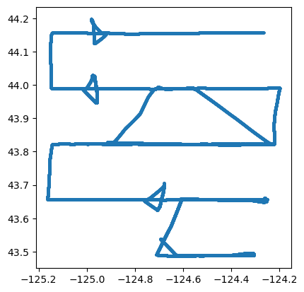

Read MVBS and plot track echograms for time periods corresponding to two ship tracks

Read MVBS as a concatenated dataset

Use xarray.open_mfdataset again to read and concatenate (combine) data files into a single xarray Dataset. This time, we’re reading the MVBS netCDF files.

%%time
MVBS_ds = xr.open_mfdataset(
    str(calibrated_dpath / 'MVBS_*.nc'), 
    data_vars='minimal', coords='minimal',
    combine='by_coords'
)

CPU times: user 6.77 s, sys: 601 ms, total: 7.38 s
Wall time: 20.3 s

MVBS_ds

<xarray.Dataset>
Dimensions:            (channel: 3, ping_time: 8819, echo_range: 150)
Coordinates:
  * channel            (channel) <U37 'GPT  18 kHz 009072058c8d 1-1 ES18-11' ...
  * ping_time          (ping_time) datetime64[ns] 2017-07-28T00:05:20 ... 201...
  * echo_range         (echo_range) float64 0.0 5.0 10.0 ... 735.0 740.0 745.0
Data variables:
    Sv                 (channel, ping_time, echo_range) float64 dask.array<chunksize=(3, 60, 150), meta=np.ndarray>
    frequency_nominal  (channel) float64 dask.array<chunksize=(3,), meta=np.ndarray>
Attributes:
    processing_software_name:     echopype
    processing_software_version:  0.8.1
    processing_time:              2024-03-22T16:12:57Z
    processing_function:          commongrid.compute_MVBS

xarray.Dataset

• Dimensions:
  • channel: 3
  • ping_time: 8819
  • echo_range: 150
• Coordinates: (3)
  • channel
    (channel)
    <U37
    'GPT 18 kHz 009072058c8d 1-1 ES...

    long_name :

    Vendor channel ID

    array(['GPT  18 kHz 009072058c8d 1-1 ES18-11',
           'GPT  38 kHz 009072058146 2-1 ES38B',
           'GPT 120 kHz 00907205a6d0 4-1 ES120-7C'], dtype='<U37')

  • ping_time
    (ping_time)
    datetime64[ns]
    2017-07-28T00:05:20 ... 2017-07-...

    long_name :

    Ping time

    standard_name :

    time

    axis :

    T

    array(['2017-07-28T00:05:20.000000000', '2017-07-28T00:05:40.000000000',
           '2017-07-28T00:06:00.000000000', ..., '2017-07-30T00:17:00.000000000',
           '2017-07-30T00:17:20.000000000', '2017-07-30T00:17:40.000000000'],
          dtype='datetime64[ns]')

  • echo_range
    (echo_range)
    float64
    0.0 5.0 10.0 ... 735.0 740.0 745.0

    long_name :

    Range distance

    units :

    m

    array([  0.,   5.,  10.,  15.,  20.,  25.,  30.,  35.,  40.,  45.,  50.,  55.,
            60.,  65.,  70.,  75.,  80.,  85.,  90.,  95., 100., 105., 110., 115.,
           120., 125., 130., 135., 140., 145., 150., 155., 160., 165., 170., 175.,
           180., 185., 190., 195., 200., 205., 210., 215., 220., 225., 230., 235.,
           240., 245., 250., 255., 260., 265., 270., 275., 280., 285., 290., 295.,
           300., 305., 310., 315., 320., 325., 330., 335., 340., 345., 350., 355.,
           360., 365., 370., 375., 380., 385., 390., 395., 400., 405., 410., 415.,
           420., 425., 430., 435., 440., 445., 450., 455., 460., 465., 470., 475.,
           480., 485., 490., 495., 500., 505., 510., 515., 520., 525., 530., 535.,
           540., 545., 550., 555., 560., 565., 570., 575., 580., 585., 590., 595.,
           600., 605., 610., 615., 620., 625., 630., 635., 640., 645., 650., 655.,
           660., 665., 670., 675., 680., 685., 690., 695., 700., 705., 710., 715.,
           720., 725., 730., 735., 740., 745.])

• Data variables: (2)
  • Sv
    (channel, ping_time, echo_range)
    float64
    dask.array<chunksize=(3, 60, 150), meta=np.ndarray>

    long_name :

    Mean volume backscattering strength (MVBS, mean Sv re 1 m-1)

    units :

    dB

    actual_range :

    [-98.92 -1.67]

    cell_methods :

    ping_time: mean (interval: 20 second comment: ping_time is the interval start) echo_range: mean (interval: 5 meter comment: echo_range is the interval start)

    binning_mode :

    physical units

    range_meter_interval :

    5m

    ping_time_interval :

    20s

    Array Chunk Bytes 30.28 MiB 362.11 kiB Shape (3, 8819, 150) (3, 103, 150) Dask graph 170 chunks in 341 graph layers Data type float64 numpy.ndarray

  • frequency_nominal
    (channel)
    float64
    dask.array<chunksize=(3,), meta=np.ndarray>

    units :

    Hz

    long_name :

    Transducer frequency

    valid_min :

    0.0

    standard_name :

    sound_frequency

    Array Chunk Bytes 24 B 24 B Shape (3,) (3,) Dask graph 1 chunks in 845 graph layers Data type float64 numpy.ndarray

• Indexes: (3)
  • channel
    PandasIndex

    PandasIndex(Index(['GPT  18 kHz 009072058c8d 1-1 ES18-11',
           'GPT  38 kHz 009072058146 2-1 ES38B',
           'GPT 120 kHz 00907205a6d0 4-1 ES120-7C'],
          dtype='object', name='channel'))

  • ping_time
    PandasIndex

    PandasIndex(DatetimeIndex(['2017-07-28 00:05:20', '2017-07-28 00:05:40',
                   '2017-07-28 00:06:00', '2017-07-28 00:06:20',
                   '2017-07-28 00:06:40', '2017-07-28 00:07:00',
                   '2017-07-28 00:07:20', '2017-07-28 00:07:40',
                   '2017-07-28 00:08:00', '2017-07-28 00:08:20',
                   ...
                   '2017-07-30 00:14:40', '2017-07-30 00:15:00',
                   '2017-07-30 00:15:20', '2017-07-30 00:15:40',
                   '2017-07-30 00:16:00', '2017-07-30 00:16:20',
                   '2017-07-30 00:16:40', '2017-07-30 00:17:00',
                   '2017-07-30 00:17:20', '2017-07-30 00:17:40'],
                  dtype='datetime64[ns]', name='ping_time', length=8819, freq=None))

  • echo_range
    PandasIndex

    PandasIndex(Float64Index([  0.0,   5.0,  10.0,  15.0,  20.0,  25.0,  30.0,  35.0,  40.0,
                   45.0,
                  ...
                  700.0, 705.0, 710.0, 715.0, 720.0, 725.0, 730.0, 735.0, 740.0,
                  745.0],
                 dtype='float64', name='echo_range', length=150))

• Attributes: (4)

  processing_software_name :

  echopype

  processing_software_version :

  0.8.1

  processing_time :

  2024-03-22T16:12:57Z

  processing_function :

  commongrid.compute_MVBS

Replace the channel dimension and coordinate with the frequency_nominal variable containing actual frequency values. Note that this step is possible only because there are no duplicated frequencies present.

%%time
MVBS_ds = ep.consolidate.swap_dims_channel_frequency(MVBS_ds)

CPU times: user 1.54 s, sys: 193 ms, total: 1.74 s
Wall time: 11.6 s

MVBS_ds

<xarray.Dataset>
Dimensions:            (frequency_nominal: 3, ping_time: 8819, echo_range: 150)
Coordinates:
  * ping_time          (ping_time) datetime64[ns] 2017-07-28T00:05:20 ... 201...
  * echo_range         (echo_range) float64 0.0 5.0 10.0 ... 735.0 740.0 745.0
  * frequency_nominal  (frequency_nominal) float64 1.8e+04 3.8e+04 1.2e+05
Data variables:
    Sv                 (frequency_nominal, ping_time, echo_range) float64 dask.array<chunksize=(3, 60, 150), meta=np.ndarray>
    channel            (frequency_nominal) <U37 'GPT  18 kHz 009072058c8d 1-1...
Attributes:
    processing_software_name:     echopype
    processing_software_version:  0.8.1
    processing_time:              2024-03-22T16:12:57Z
    processing_function:          commongrid.compute_MVBS

xarray.Dataset

• Dimensions:
  • frequency_nominal: 3
  • ping_time: 8819
  • echo_range: 150
• Coordinates: (3)
  • ping_time
    (ping_time)
    datetime64[ns]
    2017-07-28T00:05:20 ... 2017-07-...

    long_name :

    Ping time

    standard_name :

    time

    axis :

    T

    array(['2017-07-28T00:05:20.000000000', '2017-07-28T00:05:40.000000000',
           '2017-07-28T00:06:00.000000000', ..., '2017-07-30T00:17:00.000000000',
           '2017-07-30T00:17:20.000000000', '2017-07-30T00:17:40.000000000'],
          dtype='datetime64[ns]')

  • echo_range
    (echo_range)
    float64
    0.0 5.0 10.0 ... 735.0 740.0 745.0

    long_name :

    Range distance

    units :

    m

    array([  0.,   5.,  10.,  15.,  20.,  25.,  30.,  35.,  40.,  45.,  50.,  55.,
            60.,  65.,  70.,  75.,  80.,  85.,  90.,  95., 100., 105., 110., 115.,
           120., 125., 130., 135., 140., 145., 150., 155., 160., 165., 170., 175.,
           180., 185., 190., 195., 200., 205., 210., 215., 220., 225., 230., 235.,
           240., 245., 250., 255., 260., 265., 270., 275., 280., 285., 290., 295.,
           300., 305., 310., 315., 320., 325., 330., 335., 340., 345., 350., 355.,
           360., 365., 370., 375., 380., 385., 390., 395., 400., 405., 410., 415.,
           420., 425., 430., 435., 440., 445., 450., 455., 460., 465., 470., 475.,
           480., 485., 490., 495., 500., 505., 510., 515., 520., 525., 530., 535.,
           540., 545., 550., 555., 560., 565., 570., 575., 580., 585., 590., 595.,
           600., 605., 610., 615., 620., 625., 630., 635., 640., 645., 650., 655.,
           660., 665., 670., 675., 680., 685., 690., 695., 700., 705., 710., 715.,
           720., 725., 730., 735., 740., 745.])

  • frequency_nominal
    (frequency_nominal)
    float64
    1.8e+04 3.8e+04 1.2e+05

    units :

    Hz

    long_name :

    Transducer frequency

    valid_min :

    0.0

    standard_name :

    sound_frequency

    array([ 18000.,  38000., 120000.])

• Data variables: (2)
  • Sv
    (frequency_nominal, ping_time, echo_range)
    float64
    dask.array<chunksize=(3, 60, 150), meta=np.ndarray>

    long_name :

    Mean volume backscattering strength (MVBS, mean Sv re 1 m-1)

    units :

    dB

    actual_range :

    [-98.92 -1.67]

    cell_methods :

    ping_time: mean (interval: 20 second comment: ping_time is the interval start) echo_range: mean (interval: 5 meter comment: echo_range is the interval start)

    binning_mode :

    physical units

    range_meter_interval :

    5m

    ping_time_interval :

    20s

    Array Chunk Bytes 30.28 MiB 362.11 kiB Shape (3, 8819, 150) (3, 103, 150) Dask graph 170 chunks in 341 graph layers Data type float64 numpy.ndarray

  • channel
    (frequency_nominal)
    <U37
    'GPT 18 kHz 009072058c8d 1-1 ES...

    long_name :

    Vendor channel ID

    array(['GPT  18 kHz 009072058c8d 1-1 ES18-11',
           'GPT  38 kHz 009072058146 2-1 ES38B',
           'GPT 120 kHz 00907205a6d0 4-1 ES120-7C'], dtype='<U37')

• Indexes: (3)
  • ping_time
    PandasIndex

    PandasIndex(DatetimeIndex(['2017-07-28 00:05:20', '2017-07-28 00:05:40',
                   '2017-07-28 00:06:00', '2017-07-28 00:06:20',
                   '2017-07-28 00:06:40', '2017-07-28 00:07:00',
                   '2017-07-28 00:07:20', '2017-07-28 00:07:40',
                   '2017-07-28 00:08:00', '2017-07-28 00:08:20',
                   ...
                   '2017-07-30 00:14:40', '2017-07-30 00:15:00',
                   '2017-07-30 00:15:20', '2017-07-30 00:15:40',
                   '2017-07-30 00:16:00', '2017-07-30 00:16:20',
                   '2017-07-30 00:16:40', '2017-07-30 00:17:00',
                   '2017-07-30 00:17:20', '2017-07-30 00:17:40'],
                  dtype='datetime64[ns]', name='ping_time', length=8819, freq=None))

  • echo_range
    PandasIndex

    PandasIndex(Float64Index([  0.0,   5.0,  10.0,  15.0,  20.0,  25.0,  30.0,  35.0,  40.0,
                   45.0,
                  ...
                  700.0, 705.0, 710.0, 715.0, 720.0, 725.0, 730.0, 735.0, 740.0,
                  745.0],
                 dtype='float64', name='echo_range', length=150))

  • frequency_nominal
    PandasIndex

    PandasIndex(Float64Index([18000.0, 38000.0, 120000.0], dtype='float64', name='frequency_nominal'))

• Attributes: (4)

  processing_software_name :

  echopype

  processing_software_version :

  0.8.1

  processing_time :

  2024-03-22T16:12:57Z

  processing_function :

  commongrid.compute_MVBS

Extract MVBS along two N-S tracks selected via geographical bounding boxes

Define rectangular bounding boxes around two tracks oriented North-South, then plot a reference map showing all the GPS points (in red), the two bounding boxes (black), and the OOI mooring location (CE04 Oregon Offshore, yellow star) examined in the accompanying Jupyter notebook.

tracksouth_bbox = gpd.GeoSeries(box(-125.17, 43.65, -125.14, 43.84), crs=gps_gdf.crs)
tracknorth_bbox = gpd.GeoSeries(box(-125.17, 43.98, -125.14, 44.17), crs=gps_gdf.crs)

basemap = cimgt.OSM()

_, ax = plt.subplots(
    figsize=(7, 7), subplot_kw={"projection": basemap.crs}
)
bnd = gps_gdf.geometry.bounds
ax.set_extent([bnd.minx.min() - 1, bnd.maxx.max() + 2, 
               bnd.miny.min() - 0.8, bnd.maxy.max() + 2.2])
ax.add_image(basemap, 7)
ax.gridlines(draw_labels=True, xformatter=LONGITUDE_FORMATTER, yformatter=LATITUDE_FORMATTER)

# GPS points
gps_gdf.plot(ax=ax, markersize=0.1, color='red', 
             transform=ccrs.PlateCarree())

# Bounding box for selected tracks
tracksouth_bbox.plot(ax=ax, edgecolor="black", linewidth=1.2, facecolor='none', 
                     transform=ccrs.PlateCarree())
tracknorth_bbox.plot(ax=ax, edgecolor="black", linewidth=1.2, facecolor='none', 
                     transform=ccrs.PlateCarree())

# OOI CE04 Oregon Offshore mooring location
plt.plot(-124.95, 44.37, marker='*', color='yellow', markersize=13, 
         transform=ccrs.PlateCarree());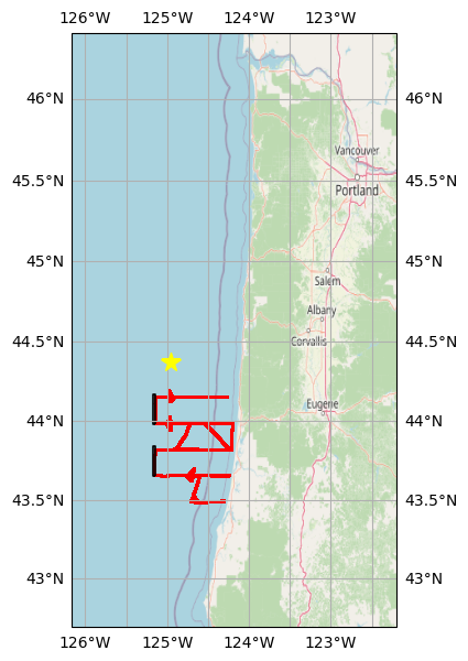

Clip the GPS locations GeoPandas GeoDataFrame gps_gdf generated from the Platform group with the two rectangular regions, tracksouth_bbox and tracknorth_bbox. Extract from those clipped GeoDataFrames (tracksouth_gps_gdf and tracknorth_gps_gdf) the minimum and maximum time1 timestamps for each track and use them to select the corresponding time span in the MVBS data.

Finally, create a MVBS Dataset subset for each track (tracksouth_MVBS_ds and tracknorth_MVBS_ds) by taking advantage of xarray’s “label”-based selection capability via the sel method. We select MVBS_ds data with ping_time values within the timestamp interval “slice” extracted from the geographical track. As we can see above, ping_time is a coordinate variable in the MVBS_ds Dataset.

tracksouth_gps_gdf = gpd.clip(gps_gdf, tracksouth_bbox)
tracksouth_MVBS_ds = MVBS_ds.sel(
    ping_time=slice(tracksouth_gps_gdf.index.min(), tracksouth_gps_gdf.index.max())
)

tracknorth_gps_gdf = gpd.clip(gps_gdf, tracknorth_bbox)
tracknorth_MVBS_ds = MVBS_ds.sel(
    ping_time=slice(tracknorth_gps_gdf.index.min(), tracknorth_gps_gdf.index.max())
)

Plot MVBS echograms for the two N-S tracks, for all 3 frequencies

The final step is to create echogram plots (range vs ping_time) for each echosounder frequency and each of the two selected ship tracks. That’s 6 subplots. We first define two functions to simplify the task. plot_echograms plots the echograms of the 3 frequencies as a column of subplots, extracting the data for each frequency by using xarray’s isel index selector method, which uses index counts rather than values. As we can see above, frequency_nominal is a coordinate of the Sv (MVBS) DataArray.

def track_interval_str(trackdt):
    """ Create the timestamp interval title string for a plot column
    """
    track_interval_title_str = (
        f"{trackdt.index.min().strftime('%b-%d %H:%MZ')}"
        f" to {trackdt.index.max().strftime('%b-%d %H:%MZ')}"
    )
    return track_interval_title_str

def plot_echograms(ds, freq_len, column_idx):
    """Plot echograms of the 3 frequencies for xarray dataset ds,
       as a column of subplots"""
    for f in range(freq_len):
        ax = axes[f][column_idx]
        # Select Sv data by frequency using the frequency_nominal coordinate index "f",
        # then plot the echogram of the selected data
        ds.Sv.isel(frequency_nominal=f).plot(
            ax=ax, 
            x='ping_time',
            y='echo_range',
            yincrease=False,
            vmin=-80,
            vmax=-50,
        )
        if f < 2:
            ax.set_xlabel(None);

freq_len = len(MVBS_ds.frequency_nominal)

fig, axes = plt.subplots(nrows=freq_len, ncols=2, constrained_layout=True, figsize=(16, 16))

fig.suptitle(
    (f"    South Track, {track_interval_str(tracksouth_gps_gdf)}"
     "                                         "
     f"North Track, {track_interval_str(tracknorth_gps_gdf)}"),
    fontsize=16)

plot_echograms(tracksouth_MVBS_ds, freq_len, column_idx=0) # left column
plot_echograms(tracknorth_MVBS_ds, freq_len, column_idx=1) # right column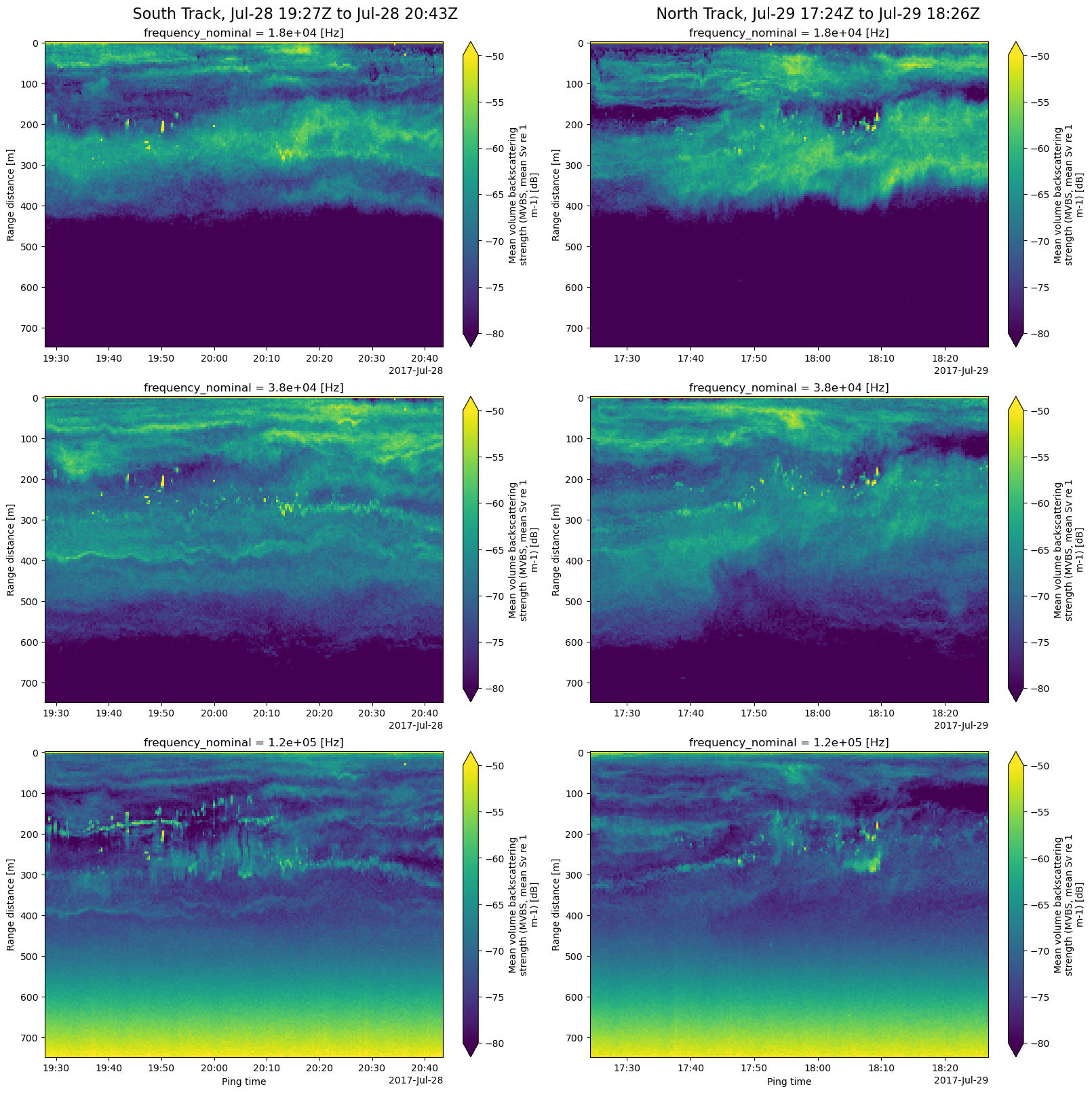

Package versions

import datetime, s3fs
print(f"echopype: {ep.__version__}, xarray: {xr.__version__}, geopandas: {gpd.__version__}, "
      f"fsspec: {fsspec.__version__}, s3fs: {s3fs.__version__}")

print(f"\n{datetime.datetime.utcnow()} +00:00")

echopype: 0.8.4, xarray: 2023.12.0, geopandas: 0.14.2, fsspec: 2023.12.2, s3fs: 2023.12.2

2024-04-26 15:56:06.174336 +00:00