library(sits)SITS - satellite image time series analysis.Loaded sits v1.5.1.
See ?sits for help, citation("sits") for use in publication.
Documentation avaliable in https://e-sensing.github.io/sitsbook/.Update: I was unable to get the code to run when I tried to run this months later.
In this example, I will use sits to prepare some imagery for a specific region and get snow estimates. https://www.usgs.gov/landsat-missions/normalized-difference-snow-index
I will use the Microsoft Planetary Computer data since it has a nice vizualization that will help me find tiles.
First step is to go to the visualizer and figure out the tiles I need. I am looking at an area close to the Canadian border of Washington state. MPC search page. I want to click on the files in the left nav and get the tile ids around “Early Winters”. I need four: “10UFU”, “10UGU”, “10UGV”, “10UFV”.
At first I used tiles, but later went to a small region of interest (roi). When I went from tiles to roi in the sits_regularize() the last date had no data and that caused errors.
library(sits)SITS - satellite image time series analysis.Loaded sits v1.5.1.
See ?sits for help, citation("sits") for use in publication.
Documentation avaliable in https://e-sensing.github.io/sitsbook/.I am going to get a month of data for a small region.
roi <- c(
  lon_min = -120.436866, lat_min = 47.570978,
  lon_max = -120.375207, lat_max = 48.611761
)
s2_cube <- sits_cube(
    source = "MPC",
    collection = "SENTINEL-2-L2A",
    roi = roi,
    bands = c("B03", "B11", "CLOUD"),
    start_date = as.Date("2022-07-01"),
    end_date = as.Date("2022-07-31")
)
  |
  |                                                                      |   0%
  |
  |===================================                                   |  50%
  |
  |======================================================================| 100%
The time line is not regular.
sits_timeline(s2_cube)Warning: cube is not regular, returning all timelines$`10TFT`
[1] "2022-07-01" "2022-07-03" "2022-07-08" "2022-07-11" "2022-07-13"
[6] "2022-07-16" "2022-07-18" "2022-07-21" "2022-07-23" "2022-07-26"
[11] "2022-07-28"
$`10UFU`
[1] "2022-07-01" "2022-07-06" "2022-07-11" "2022-07-16" "2022-07-21"
[6] "2022-07-26"The documentation says things are faster if we save a copy of our files. And we will reduce the area of interest to a really small area and weekly data. This is going to save a bunch of little files (4 tiles x 52 weeks x 3 bands) into the tempdir. This saving takes a long time itself and seems kind of pointless for this case. So I skipped this.
# roi as (lon_min, lon_max, lat_min, lat_max)
roi <- c(
  lon_min = -120.436866, lat_min = 48.570978,
  lon_max = -120.375207, lat_max = 48.611761
)
sits_cube_copy(s2_cube,
  output_dir = here::here("topics-2024/2024-05-24-sits/tempdir/chl1"),
  roi = roi
)
  |
  |                                                                      |   0%
  |
  |=                                                                     |   2%
  |
  |===                                                                   |   4%
  |
  |====                                                                  |   6%
  |
  |=====                                                                 |   8%
  |
  |=======                                                               |  10%
  |
  |========                                                              |  12%
  |
  |==========                                                            |  14%
  |
  |===========                                                           |  16%
  |
  |============                                                          |  18%
  |
  |==============                                                        |  20%
  |
  |===============                                                       |  22%
  |
  |================                                                      |  24%
  |
  |==================                                                    |  25%
  |
  |===================                                                   |  27%
  |
  |=====================                                                 |  29%
  |
  |======================                                                |  31%
  |
  |=======================                                               |  33%
  |
  |=========================                                             |  35%
  |
  |==========================                                            |  37%
  |
  |===========================                                           |  39%
  |
  |=============================                                         |  41%
  |
  |==============================                                        |  43%
  |
  |================================                                      |  45%
  |
  |=================================                                     |  47%
  |
  |==================================                                    |  49%
  |
  |====================================                                  |  51%
  |
  |=====================================                                 |  53%
  |
  |======================================                                |  55%
  |
  |========================================                              |  57%
  |
  |=========================================                             |  59%
  |
  |===========================================                           |  61%
  |
  |============================================                          |  63%
  |
  |=============================================                         |  65%
  |
  |===============================================                       |  67%
  |
  |================================================                      |  69%
  |
  |=================================================                     |  71%
  |
  |===================================================                   |  73%
  |
  |====================================================                  |  75%
  |
  |======================================================                |  76%
  |
  |=======================================================               |  78%
  |
  |========================================================              |  80%
  |
  |==========================================================            |  82%
  |
  |===========================================================           |  84%
  |
  |============================================================          |  86%
  |
  |==============================================================        |  88%
  |
  |===============================================================       |  90%
  |
  |=================================================================     |  92%
  |
  |==================================================================    |  94%
  |
  |===================================================================   |  96%
  |
  |===================================================================== |  98%
  |
  |======================================================================| 100%
# A tibble: 2 × 12
source collection satellite sensor tile xmin xmax ymin ymax crs
<chr> <chr> <chr> <chr> <chr> <dbl> <dbl> <dbl> <dbl> <chr>
1 MPC SENTINEL-2-L2A SENTINEL… MSI 10UFU 688910 693620 5.38e6 5.39e6 EPSG…
2 MPC SENTINEL-2-L2A SENTINEL… MSI 10UFU 688900 693620 5.38e6 5.39e6 EPSG…
# ℹ 2 more variables: labels <list>, file_info <list>Next we need to regularize our cube. I will regularize to 14 day period with a 60m resolution. This is going to take a little while time.
reg_cube <- sits_regularize(
  cube = s2_cube,
  output_dir = here::here("topics-2024/2024-05-24-sits/tempdir/chl2"),
  roi = roi,
  res  = 60,
  period = "P14D",
  multicores = 4
 )
Warning: regularization is faster when data is stored locally
use 'sits_cube_copy()' to copy data locally before regularization
  |
  |                                                                      |   0%
  |
  |===================================                                   |  50%
  |
|======================================================================| 100%https://sentiwiki.copernicus.eu/web/s2-processing#S2Processing-Step1b:NormalisedDifferenceSnowIndex(NDSI)
reg_cube <- sits_apply(reg_cube,
   NDSI = (B03 - B11)/(B03 + B11),
   output_dir = here::here("topics-2024/2024-05-24-sits/tempdir/chl2"),
   multicores = 4
)Make a plot.
plot(reg_cube,
  band = "NDSI",
  date = "2022-07-15"
)
-- tmap v3 code detected --[v3->v4] tm_raster(): instead of 'style = "cont"', use 'col.scale = tm_scale_continuous()' and migrate the argument(s) 'style.args', 'midpoint', 'palette' (rename to 'values') to 'tm_scale_continuous(<HERE>)'. For small multiples, specify a 'tm_scale_' for each multiple, and put them in a list: 'col.scale = list(<scale1>, <scale2>, ...)'[v3->v4] tm_raster(): migrate the argument(s) related to the legend of the visual variable 'col', namely 'title' to 'col.legend = tm_legend(<HERE>)'[cols4all] color palettes: use palettes from the R package cols4all. Run 'cols4all::c4a_gui()' to explore them. The old palette name "RdYlGn" is named "rd_yl_gn" (in long format "brewer.rd_yl_gn")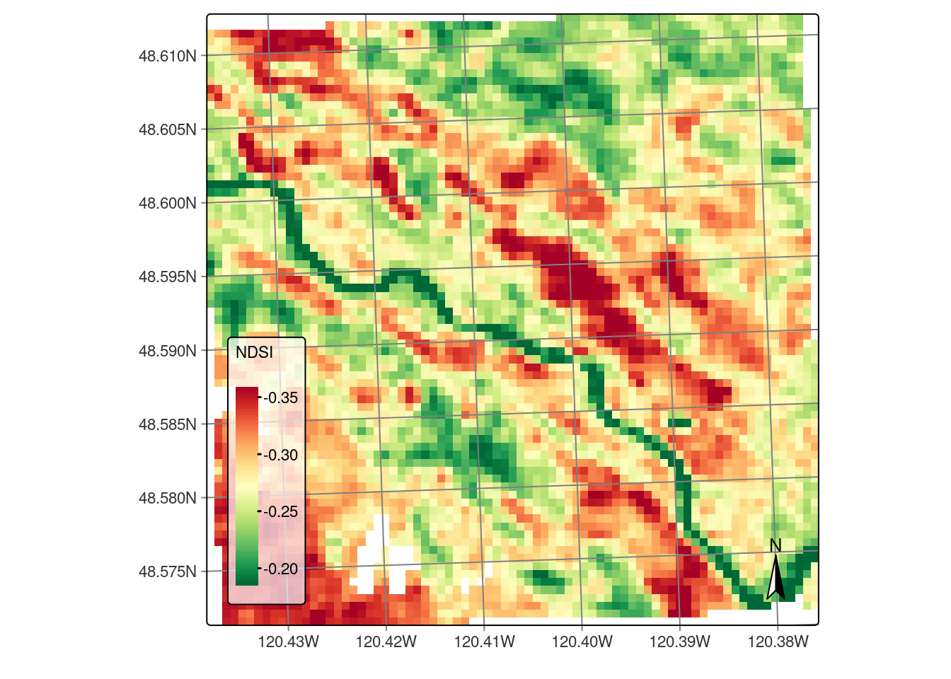
ERROR
# Obtain a time series from the raster cube from a point
sample_latlong <- tibble::tibble(
  longitude = -120.43687,
  latitude  = -47.57098
)
series <- sits_get_data(
  cube = reg_cube,
  samples = sample_latlong
)