import earthaccess
import xarray as xrEarthdata Search and Discovery
📘 Learning Objectives
- How to authenticate with
earthaccess- How to use
earthaccessto search for data using spatial and temporal filters- How to explore and work with search results
- How to plot a single file
Summary
In this example we will use the earthaccess library to search for data collections from NASA Earthdata. earthaccess is a Python library that simplifies data discovery and access to NASA Earth science data by providing an abstraction layer for NASA’s Common Metadata Repository (CMR) API Search API. The library makes searching for data more approachable by using a simpler notation instead of low level HTTP queries. earthaccess takes the trouble out of Earthdata Login authentication, makes search easier, and provides a stream-line way to download or stream search results into an xarray object.
For more on earthaccess visit the earthaccess GitHub page and/or the earthaccess documentation site. Be aware that earthaccess is under active development.
Prerequisites
An Earthdata Login account is required to access data from NASA Earthdata. Please visit https://urs.earthdata.nasa.gov to register and manage your Earthdata Login account. This account is free to create and only takes a moment to set up.
Get Started
Import Required Packages
auth = earthaccess.login()
# are we authenticated?
if not auth.authenticated:
    # ask for credentials and persist them in a .netrc file
    auth.login(strategy="interactive", persist=True)
Search for data
We want to search NASA Earthdata for collections using the OCI instrument. Use https://search.earthdata.nasa.gov/search?fi=OCI
There are multiple keywords we can use to discovery data from collections. The table below contains the short_name, concept_id, and doi for some collections we are interested in for other exercises. Each of these can be used to search for data or information related to the collection we are interested in.
| Description | Shortname | Collection Concept ID |
|---|---|---|
| Level 2 Apparent Optical Properties | PACE_OCI_L2_AOP | C3385049983-OB_CLOUD |
| Level 3 RRS | PACE_OCI_L3M_RRS | C3385050676-OB_CLOUD |
How can we find the shortname or concept_id for collections not in the table above?. Let’s take a quick detour.
Search by collection - Level 2 data
# Level 2 data
results = earthaccess.search_data(
    short_name = 'PACE_OCI_L2_AOP',
    temporal = ("2025-03-05", "2025-03-05")
)
len(results)143Why are there so many?? Level 2 data is swath data and swath data is in spatial chunks. We need to specify a bounding box.
# Level 2 data
results = earthaccess.search_data(
    short_name = 'PACE_OCI_L2_AOP',
    temporal = ("2025-03-05", "2025-03-05"),
    bounding_box = (-98.0, 27.0, -96.0, 31.0)
)
len(results)1Search by collection - Level 3 data
Level 3 is global data (no swaths and no tiles) so there should be one file per day, right?
# Level 3 data
results = earthaccess.search_data(
    short_name = 'PACE_OCI_L3M_RRS',
    temporal = ("2025-03-05", "2025-03-05")
)
len(results)6Why so many? There are month, 8-day, day and 2 resolutions. You need to look at the filenames and filter to get the files you want.
# all the file names
[res.data_links() for res in results]
[['https://obdaac-tea.earthdatacloud.nasa.gov/ob-cumulus-prod-public/PACE_OCI.20250226_20250305.L3m.8D.RRS.V3_0.Rrs.0p1deg.nc'],
['https://obdaac-tea.earthdatacloud.nasa.gov/ob-cumulus-prod-public/PACE_OCI.20250226_20250305.L3m.8D.RRS.V3_0.Rrs.4km.nc'],
['https://obdaac-tea.earthdatacloud.nasa.gov/ob-cumulus-prod-public/PACE_OCI.20250301_20250331.L3m.MO.RRS.V3_0.Rrs.4km.nc'],
['https://obdaac-tea.earthdatacloud.nasa.gov/ob-cumulus-prod-public/PACE_OCI.20250301_20250331.L3m.MO.RRS.V3_0.Rrs.0p1deg.nc'],
['https://obdaac-tea.earthdatacloud.nasa.gov/ob-cumulus-prod-public/PACE_OCI.20250305.L3m.DAY.RRS.V3_0.Rrs.0p1deg.nc'],
['https://obdaac-tea.earthdatacloud.nasa.gov/ob-cumulus-prod-public/PACE_OCI.20250305.L3m.DAY.RRS.V3_0.Rrs.4km.nc']]# Level 3 data
results = earthaccess.search_data(
short_name = 'PACE_OCI_L3M_RRS',
temporal = ("2025-03-05", "2025-03-05"),
granule_name="*.MO.*.0p1deg.*"
)
len(results)1Refining the search
Here are the common arguments for earthaccess.search_data():
bounding_boxis a lat/lon box, e.g.(xmin=-73.5, ymin=33.5, xmax=-43.5, ymax=43.5)temporalis a date range, e.g.("2020-01-16", "2020-12-16")cloud_coveris a range(0, 10)granule_nameis a matching filter, e.g."*.DAY.*.0p1deg.*"short_nameorcollection_id
Working with earthaccess returns
Following the search for data, you’ll likely take one of two pathways with those results. You may choose to download the assets that have been returned to you or you may choose to continue working with the search results within the Python environment.
type(results[0])earthaccess.results.DataGranuleresults[0]Download earthaccess results
In some cases you may want to download your assets. earthaccess makes downloading the data from the search results very easy using the earthaccess.download() function.
downloaded_files = earthaccess.download( results[0:9], local_path=‘data’, )
earthaccess does a lot of heavy lifting for us. It identifies the downloadable links, passes our Earthdata Login credentials, and saves the files with the proper names.
Work in the cloud
Alternatively we can work with the metadata without downloading and only load the data into memory (or download) when we need to compute with it or plot it. We use earthaccess‘s open() method to create a ’fileset’ to the cloud objects and then open that with xarray.
fileset = earthaccess.open(results)ds = xr.open_dataset(fileset[0], chunks={})
ds<xarray.Dataset> Size: 4GB
Dimensions: (wavelength: 172, lat: 1800, lon: 3600, rgb: 3,
eightbitcolor: 256)
Coordinates:
* wavelength (wavelength) float64 1kB 346.0 348.0 351.0 ... 714.0 717.0 719.0
* lat (lat) float32 7kB 89.95 89.85 89.75 ... -89.75 -89.85 -89.95
* lon (lon) float32 14kB -179.9 -179.9 -179.8 ... 179.8 179.9 180.0
Dimensions without coordinates: rgb, eightbitcolor
Data variables:
Rrs (lat, lon, wavelength) float32 4GB dask.array<chunksize=(16, 1024, 8), meta=np.ndarray>
palette (rgb, eightbitcolor) uint8 768B dask.array<chunksize=(3, 256), meta=np.ndarray>
Attributes: (12/64)
product_name: PACE_OCI.20250226_20250305.L3m.8D.RRS....
instrument: OCI
title: OCI Level-3 Standard Mapped Image
project: Ocean Biology Processing Group (NASA/G...
platform: PACE
source: satellite observations from OCI-PACE
... ...
identifier_product_doi: 10.5067/PACE/OCI/L3M/RRS/3.0
keywords: Earth Science > Oceans > Ocean Optics ...
keywords_vocabulary: NASA Global Change Master Directory (G...
data_bins: 2431585
data_minimum: -0.010000002
data_maximum: 0.10000001ds_size_gb = ds.nbytes / 1e9
print(f"Dataset size: {ds_size_gb:.2f} GB")Dataset size: 4.46 GBWe can plot this object.
rrs = ds['Rrs'].sel(wavelength=346, lat=slice(47, 25), lon=slice(-98, -66))
rrs.plot();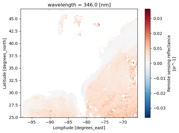
Chunks
The data are cloud-optimized (read optimized) so that we don’t have to read the whole file into memory to work with it and we don’t have to download the whole thing if we don’t need to.
ds.chunksFrozen({'lat': (16, 16, 16, 16, 16, 16, 16, 16, 16, 16, 16, 16, 16, 16, 16, 16, 16, 16, 16, 16, 16, 16, 16, 16, 16, 16, 16, 16, 16, 16, 16, 16, 16, 16, 16, 16, 16, 16, 16, 16, 16, 16, 16, 16, 16, 16, 16, 16, 16, 16, 16, 16, 16, 16, 16, 16, 16, 16, 16, 16, 16, 16, 16, 16, 16, 16, 16, 16, 16, 16, 16, 16, 16, 16, 16, 16, 16, 16, 16, 16, 16, 16, 16, 16, 16, 16, 16, 16, 16, 16, 16, 16, 16, 16, 16, 16, 16, 16, 16, 16, 16, 16, 16, 16, 16, 16, 16, 16, 16, 16, 16, 16, 8), 'lon': (1024, 1024, 1024, 528), 'wavelength': (8, 8, 8, 8, 8, 8, 8, 8, 8, 8, 8, 8, 8, 8, 8, 8, 8, 8, 8, 8, 8, 4), 'rgb': (3,), 'eightbitcolor': (256,)})Chunking let’s us work with big datasets without blowing up our memory. This task takes awhile but it doesn’t blow up our little 2Gb RAM virtual machines. xarray and dask are smart and work through the task chunk by chunk.
%%time
# Pick a variable and a wavelength value
varname = list(ds.data_vars)[0]
# select the first wavelength
one_wl = ds[varname].isel(wavelength=0)
# under the hood, dask + xarray is computing the mean chunk by chunk
val = one_wl.mean(dim=("lat", "lon")).compute()
If we tried to load the data into memory, we would crash our kernel (max out the RAM).
%%time
# THIS WILL CRASH THE KERNEL
# this tries to load the whole dataset all at once into memory
unchunked_slice = one_wl.load()
# this would be fast if the load step didn't crash the memory
val = unchunked_slice.mean(dim=("lat", "lon"))
Summary
This concludes tutorial 1. You have worked with some PACE data in the cloud and plotted a single file.