Extract data within a boundary

Learning Objectives

How to access and download sea surface temperature from NASA Earthdata
How to apply shapefiles as masks to satellite data
How to compute monthly average sea surface temperature

Summary

In this example, we will utilize the earthdatalogin R package to retrieve sea surface temperature data from NASA Earthdata search. The earthdatalogin R package simplifies the process of discovering and accessing NASA Earth science data.

This example is adapted from the NOAA CoastWatch Satellite Data Tutorials. To explore the full range of tutorials on accessing and utilizing oceanographic satellite data, visit the NOAA CoastWatch Tutorial Github repository.

For more on earthdatalogin visit the earthdatalogin GitHub page and/or the earthdatalogin documentation site. Be aware that earthdatalogin is under active development and that we are using the development version on GitHub.

Terminology

shapefiles: is a simple, nontopological format for storing the geometric location and attribute information of geographic features. Geographic features in a shapefile can be represented by points, lines, or polygons (areas). Learn more here.

Prerequisites

The tutorials today can be run with the guest Earthdata Login that is in earthdatalogin. However, if you will be using the NASA Earthdata portal more regularly, please register for an Earthdata Login account. Please https://urs.earthdata.nasa.gov to register and manage your Earthdata Login account. This account is free to create and only takes a moment to set up.

Import Required Packages

Note: See the set-up tab (in left nav bar) for instructions on getting set up on your own computer, but be aware that getting it is common to run into trouble getting GDAL set up properly to handle netCDF files. Using a Docker image (and Python) is often less aggravating.

Datasets used

GHRSST Level 4 AVHRR_OI Global Blended Sea Surface Temperature Analysis (GDS2) from NCEI
This NOAA blended SST is a moderate resolution satellite-based gap-free sea surface temperature (SST) product. We will use the daily data. https://cmr.earthdata.nasa.gov/search/concepts/C2036881712-POCLOUD.html

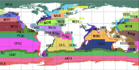
Longhurst Marine Provinces
The dataset represents the division of the world oceans into provinces as defined by Longhurst (1995; 1998; 2006). This division has been based on the prevailing role of physical forcing as a regulator of phytoplankton distribution.

The Longhurst Marine Provinces dataset is available online (https://www.marineregions.org/downloads.php) and within the shapes folder associated with this repository. For this exercise we will use the Gulf Stream province (ProvCode: GFST)

Load packages

library(terra)
library(earthdatalogin)
library(sf)
library(ggplot2)

Load boundary coordinates

The shapefile for the Longhurst marine provinces includes a list of regions.
For this exercise, we will only use the boundary of one province, the Gulf Stream region (“GFST”).

# Set directory path for shapefile
dir_path <- '../resources/longhurst_v4_2010/'

# Import shape files (Longhurst coordinates)
shapes <- sf::read_sf(dsn = dir_path, layer = "Longhurst_world_v4_2010")

# Example List of all the province names
shapes$ProvCode

 [1] "BPLR" "ARCT" "SARC" "NADR" "GFST" "NASW" "NATR" "WTRA" "ETRA" "SATL"
[11] "NECS" "CNRY" "GUIN" "GUIA" "NWCS" "MEDI" "CARB" "NASE" "BRAZ" "FKLD"
[21] "BENG" "MONS" "ISSG" "EAFR" "REDS" "ARAB" "INDE" "INDW" "AUSW" "BERS"
[31] "PSAE" "PSAW" "KURO" "NPPF" "NPSW" "TASM" "SPSG" "NPTG" "PNEC" "PEQD"
[41] "WARM" "ARCH" "ALSK" "CCAL" "CAMR" "CHIL" "CHIN" "SUND" "AUSE" "NEWZ"
[51] "SSTC" "SANT" "ANTA" "APLR"

# Get boundary coordinates for Gulf Stream region (GFST)
GFST <- shapes[shapes$ProvCode == "GFST",]

xcoord <- sf::st_coordinates(GFST)[,1]
ycoord <- sf::st_coordinates(GFST)[,2]

Search data from NASA Earthdata with the dataset unique name and coordinates/dates

First, connect to NASA Earthdata with no credentials

earthdatalogin::edl_netrc()

Then, define your search and cropping criteria

# Dataset unique name
short_name <- 'AVHRR_OI-NCEI-L4-GLOB-v2.1'

# Set boundaries based on the shapefile
bbox <- c(xmin=min(xcoord), ymin=min(ycoord), xmax=max(xcoord), ymax=max(ycoord)) 

# Set time range
tbox <- c("2020-01-01", "2020-04-01")

# Search data that match the boundaries and time range
results <- earthdatalogin::edl_search(
  short_name = short_name,
  version = "2.1",
  temporal = tbox,
  bounding_box = paste(bbox, collapse = ",")
)

# Check number of files 
length(results)

[1] 93

There are 93 files.

Apply shapefiles as mask to satellite data

# Select the first result
ras <- terra::rast(results[1], vsi = TRUE)

# Extract SST from the multi-layer raster data
ras_sst <- ras[["analysed_sst"]]

Convert shape to SpatVector for terra.

# Vectorize shapes
shp <- terra::vect(shapes)

# Get boundaries for GFST
GFST <- shp[shp$ProvCode == "GFST",]

Plot the SST data.

plot(ras_sst)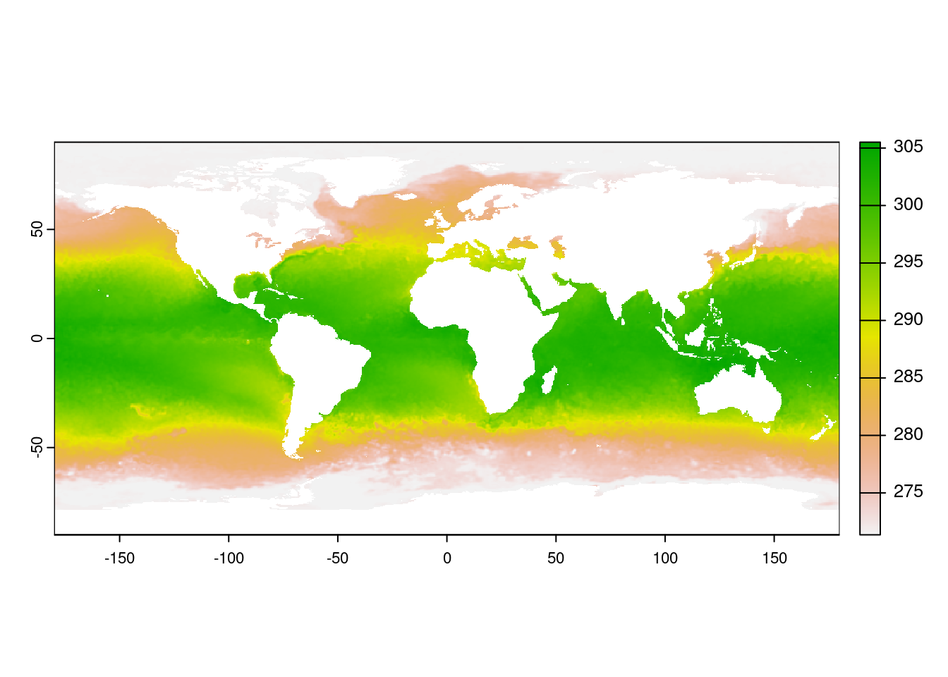

Plot GFST boundaries from shapefile.

plot(GFST,col='red')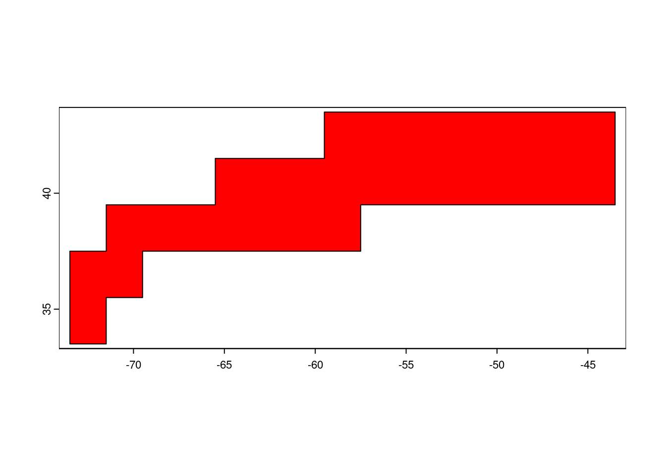

Mask SST with the GFST boundaries and plot.

masked_rc <- terra::mask(ras_sst, GFST)

# Visualize the SST in GFST Province and crop to the GFST extent
plot(masked_rc, ext = GFST)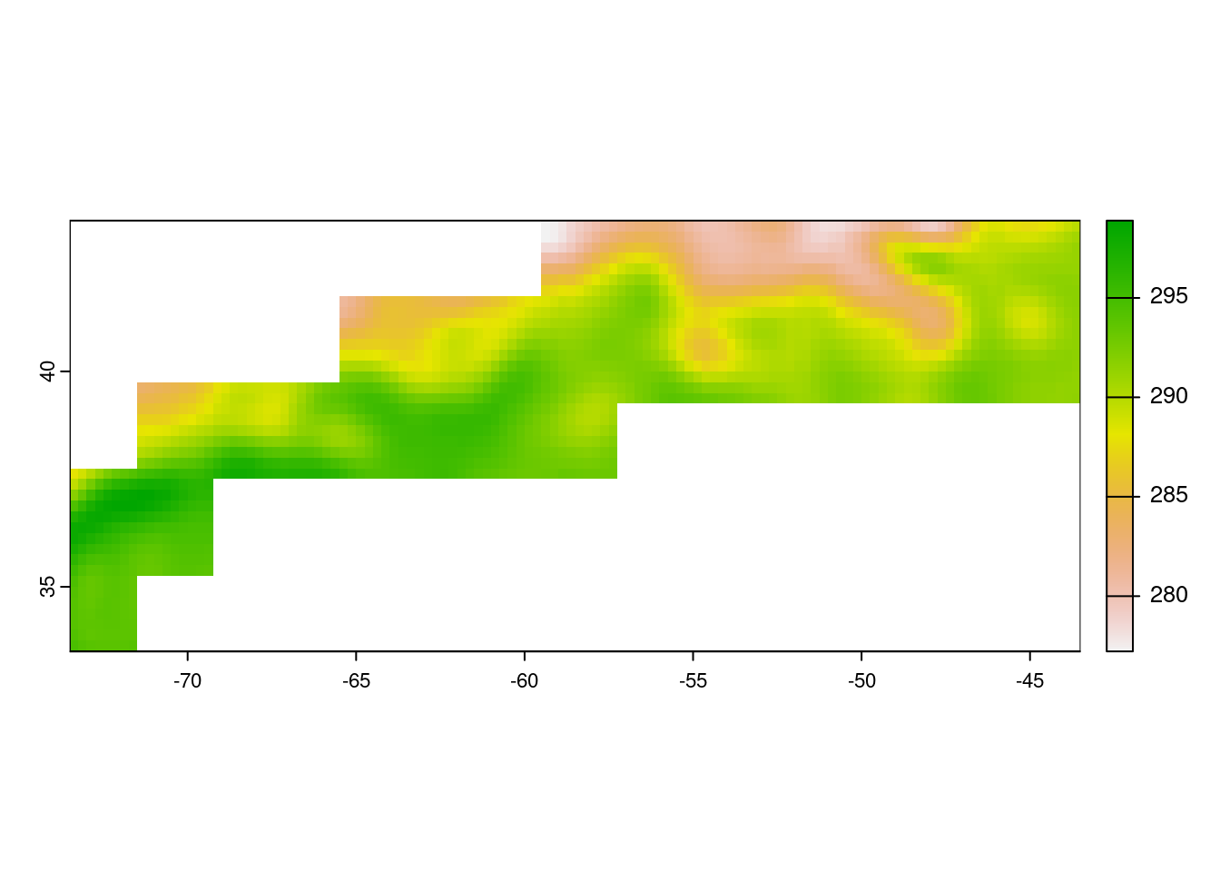

Compute monthly average of SST

We will construct a data cube to compute monthly average for sea surface temperature data within the boundary. To minimize data loading times, the first 10 results, which correspond to approximately two months of data, will be used for this exercise.

Select the first 10 SST results (end of January and beginning of February).

ras_all <- terra::rast(results[c(25:35)], vsi = TRUE)

Select SST data. The trim and mask operations are memory intensive and we want to select only the layer we will be working with.

rc_sst <- ras_all["analysed_sst",]

Crop to the GFST boundaries.

rc_sst <- terra::crop(rc_sst, GFST)

Trim the SST data to the boundaries of GFST.

rc_sst <- terra::mask(rc_sst, GFST)

Calculate mean SST over the entire time series (10 days) and map it.

raster_mean <- terra::mean(rc_sst, na.rm=TRUE)

Plot the mean SST.

plot(raster_mean)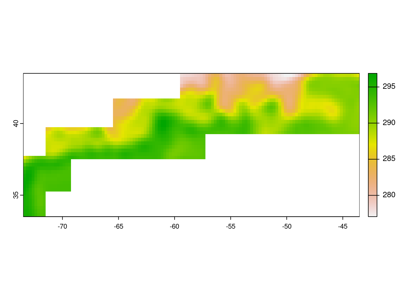

Calculate monthly mean SST means across rasters

First create a function to convert times to year-month format. This will create a vector that shows which datas are in which month-year.

year_month <- function(x) {
  format(as.Date(time(x), format="%Y-%m-%d"), "%Y-%m")
}
ym <- year_month(rc_sst)
ym

 [1] "2020-01" "2020-01" "2020-01" "2020-01" "2020-01" "2020-01" "2020-01"
 [8] "2020-01" "2020-02" "2020-02" "2020-02"

Compute raster mean grouped by Year-month. tapp is the terra equivalent of tapply and allow you to apply a function to groups of raster time layers. This allows you to do temporal aggregation. Use ?tapp to learn about this function.

monthly_mean_rast <- terra::tapp(rc_sst, ym, fun = mean)
monthly_mean_rast

class       : SpatRaster 
dimensions  : 40, 120, 2  (nrow, ncol, nlyr)
resolution  : 0.25, 0.25  (x, y)
extent      : -73.5, -43.5, 33.5, 43.5  (xmin, xmax, ymin, ymax)
coord. ref. : lon/lat WGS 84 
source(s)   : memory
names       : X2020.01, X2020.02 
min values  : 277.0425, 276.9367 
max values  : 297.1500, 296.9033

Compute mean across raster grouped by Year-month. global() applies a function to the entire raster. Use ?global to learn about this function.

monthly_means <- terra::global(monthly_mean_rast, fun = mean, na.rm=TRUE)
monthly_means

             mean
X2020.01 289.3776
X2020.02 289.0583

Convert to data frame

We convert to a data frame to plot time series.

# Convert raster into data.frame
monthly_means_df <- as.data.frame(monthly_means)

# Create a year_month column
monthly_means_df$year_month <- sub("X", "", rownames(monthly_means_df))

Plot monthly mean of sea surface temperature within GFST province

ggplot(data = monthly_means_df, aes(x = year_month, y = mean, group = 1)) +
  geom_line() +
  geom_point() +
  xlab("Year.Month") + 
  ylab("Mean SST (F)")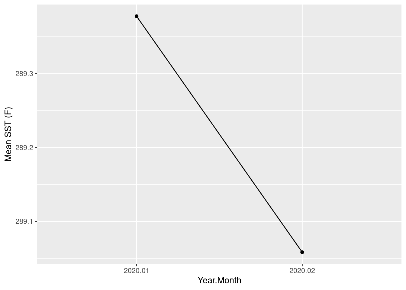

Troubleshooting

If you get the following error:

Warning: Opening a /vsi file with the netCDF driver requires Linux userfaultfd to be available. Or you may set the GDAL_SKIP=netCDF configuration option to force the use of the HDF5 driver. (GDAL error 1)Error: [rast] file does not exist: /vsicurl/https://archive.podaac.earthdata.nasa.gov/podaac-ops-cumulus-protected/AVHRR_OI-NCEI-L4-GLOB-v2.1/20191231120000-NCEI-L4_GHRSST-SSTblend-AVHRR_OI-GLOB-v02.0-fv02.1.nc

Then go back and run the authentication code at the top.