In this tutorial, we will provide a brief introduction to:
Open RStudio in the JupyterHub
Basic navigation around RStudio: the 4 main panels and menus
The help panel
Create a RStudio project
Installing packages
Uploading and downloading files
Creating files and creating files with templates
Command line (terminal/shell) in RStudio
Open RStudio in the JupyterHub
Login the JupyterHub
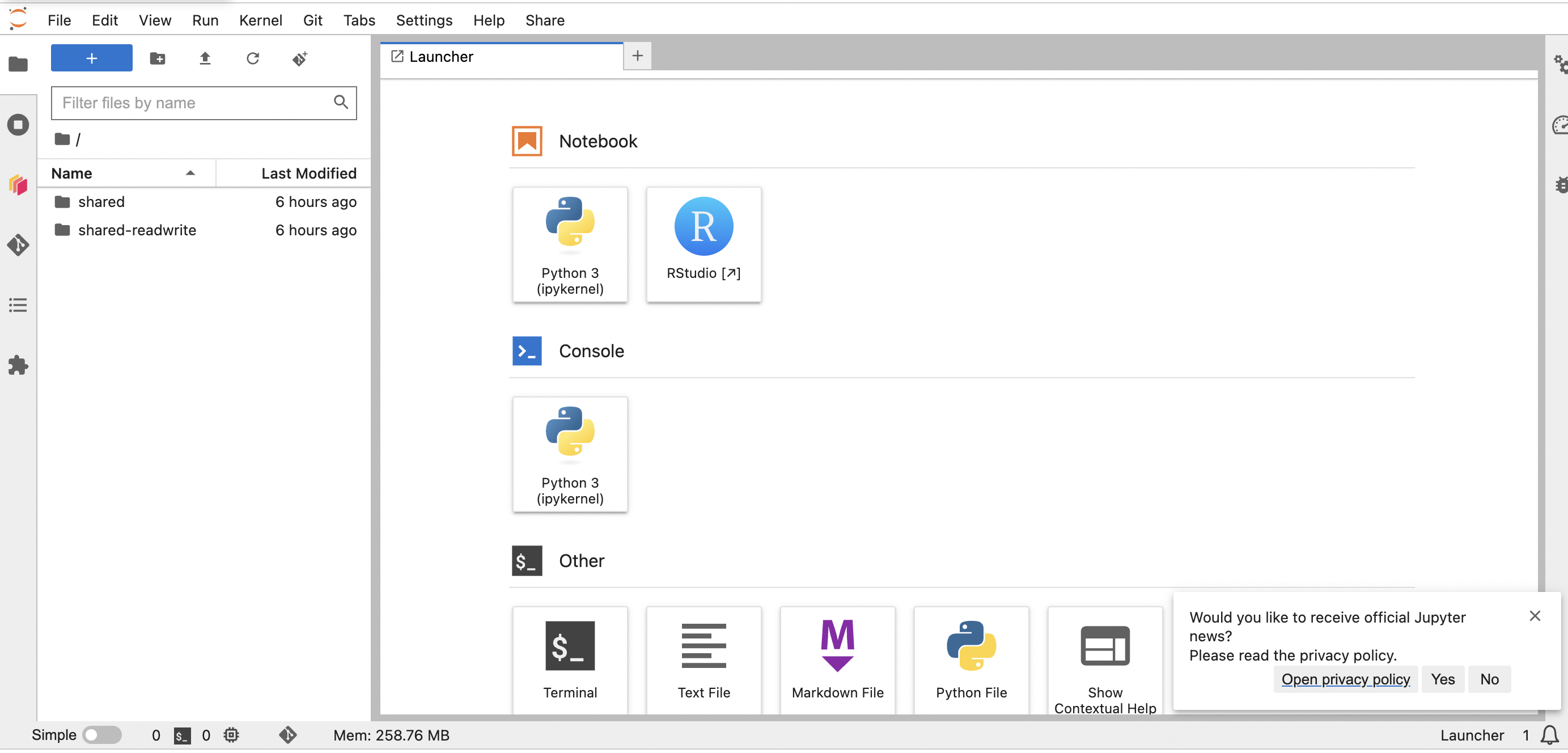
Click on the RStudio button when the Launcher appears
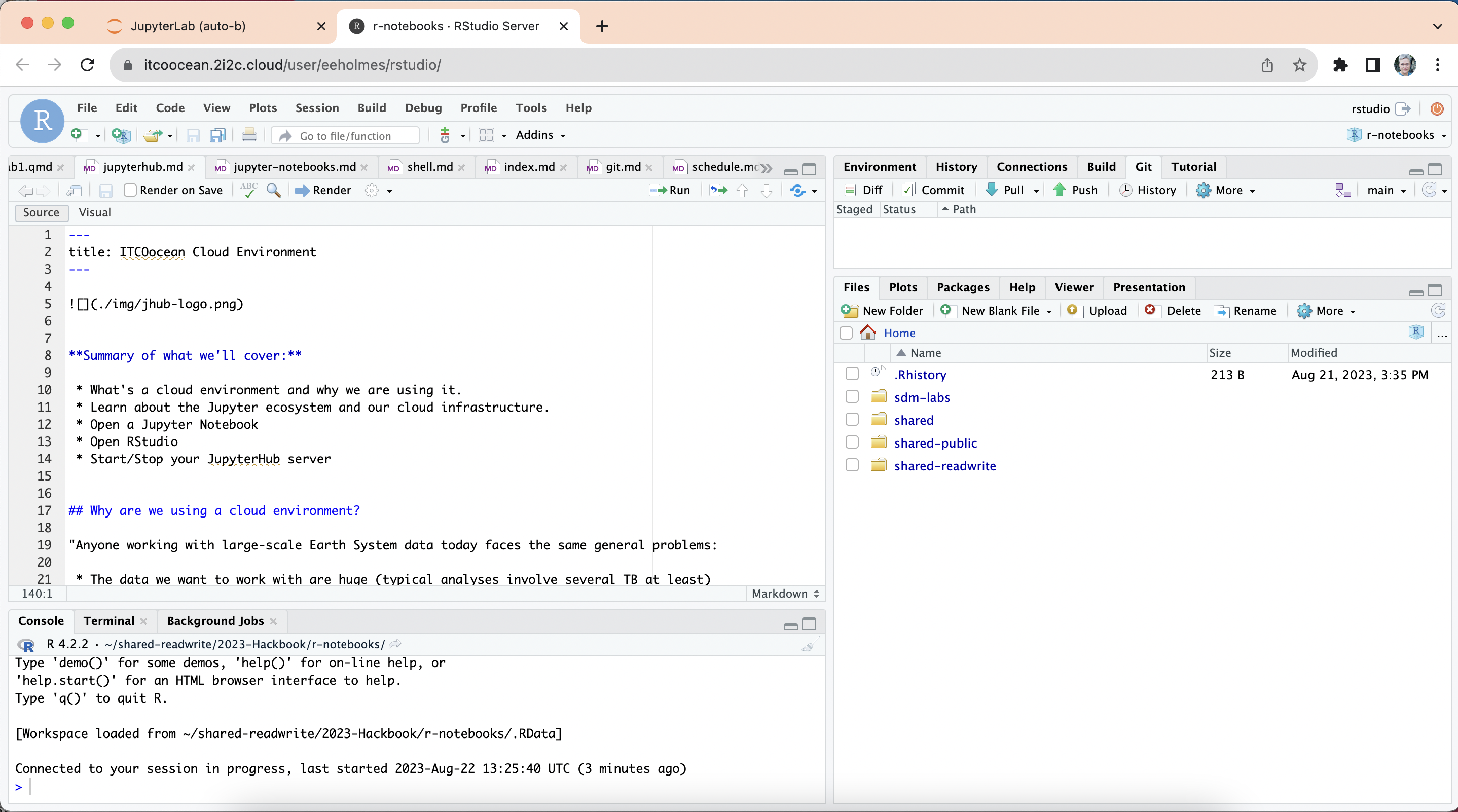
Look for the browser tab with the RStudio icon
Basic Navigation
RStudio Panels
Create an RStudio project
Open RStudio
In the file panel, click on the Home icon to make sure you are in your home directory
From the file panel, click “New Project” to create a new project
In the pop up, select New Directory and then New Project
Name it sandbox
Click on the dropdown in the upper right corner to select your sandbox project
Click on Tools > Project Options > General and change the first 2 options about saving and restoring the workspace to “No”
Installing packages
In the bottom right panel, select the Packages tab, click install and then start typing the name of the package. Then click Install.
The JupyterHub comes with many packages already installed so you shouldn’t have to install many packages.
When you want to use a package, you first need to load it with
library(hello)
You will see this in the tutorials. You might also see something like
hello::thefunction()
This is using thefunction() from the hello package.
Note
Python users. In R, you will always call a function like funtion(object) and never like object.function(). The exception is something called ‘piping’ in R, which I have never seen in Python. In this case you pass objects left to right. Like object %>% function(). Piping is very common in modern R but you won’t see it much in R from 10 years ago.
Uploading and downloading files
Note, Upload and download is only for the JupyterHub not on RStudio on your computer.
Uploading is easy.
Look for the Upload button in the Files tab of the bottom right panel.
Download is less intuitive.
Click the checkbox next to the file you want to download. One only.
Click the “cog” icon in the Files tab of the bottom right panel. Then click Export.
Creating files
When you start your server, you will have access to your own virtual drive space. No other users will be able to see or access your files. You can upload files to your virtual drive space and save files here. You can create folders to organize your files. You personal directory is home/rstudio. Everyone has the same home directory but your files are separate and cannot be seen by others.
Python users: If you open a Python image instead of the R image, your home is home/jovyan.
There are a number of different ways to create new files. Let’s practice making new files in RStudio.
R Script
Open RStudio
In the upper right, make sure you are in your sandbox project.
From the file panel, click on “New Blank File” and create a new R script.
Paste
print("Hello World")
1+1
in the script. 7. Click the Source button (upper left of your new script file) to run this code. 8. Try putting your cursor on one line and running that line of code by clicking “Run” 9. Try selecting lines of code and running that by clicking “Run”
csv file
From the file panel, click on “New Blank File” and create a Text File.
The file will open in the top left corner. Paste in the following:
name, place, value
A, 1, 2
B, 10, 20
C, 100, 200
Click the save icon (above your new file) to save your csv file
A Rmarkdown document
Now let’s create some more complicated files using the RStudio template feature.
From the upper left, click File -> New File -> RMarkdown
Click “Ok” at the bottom.
When the file opens, click Knit (icon at top of file).