SDM lab 1 - Downloading species data with robis

Here we download from OBIS using the robis package.

Set up

here::i_am("r-tutorials/SDM-lab-robis.qmd")

here() starts at /Users/eli.holmes/Documents/GitHub/NOAAHackDays

dir_data <- here::here("r-tutorials", "data")

library(ggplot2)
library(sf)

Linking to GEOS 3.11.0, GDAL 3.5.3, PROJ 9.1.0; sf_use_s2() is TRUE

library("rnaturalearth")
library("rnaturalearthdata")


Attaching package: 'rnaturalearthdata'

The following object is masked from 'package:rnaturalearth':

    countries110

library(raster)

Loading required package: sp

library(tidyverse)

── Attaching core tidyverse packages ──────────────────────── tidyverse 2.0.0 ──
✔ dplyr     1.1.3     ✔ readr     2.1.4
✔ forcats   1.0.0     ✔ stringr   1.5.0
✔ lubridate 1.9.2     ✔ tibble    3.2.1
✔ purrr     1.0.1     ✔ tidyr     1.3.0

── Conflicts ────────────────────────────────────────── tidyverse_conflicts() ──
✖ tidyr::extract() masks raster::extract()
✖ dplyr::filter()  masks stats::filter()
✖ dplyr::lag()     masks stats::lag()
✖ dplyr::select()  masks raster::select()
ℹ Use the conflicted package (<http://conflicted.r-lib.org/>) to force all conflicts to become errors

library(robis)


Attaching package: 'robis'

The following object is masked from 'package:raster':

    area

Create a bounding box

bbox <- sf::st_bbox(c(xmin = 41.875, xmax = 65.125, ymax = -0.125, ymin = 32.125), 
                          crs = sf::st_crs(4326))

Creates a sf object with a sfs_POLYGON from which we can get a polygon string. We also use this for cropping with the raster package, while we will need bbox for cropping with the stars package.

extent_polygon <-  bbox %>% sf::st_as_sfc() %>% st_sf()

Then for the robis package we need a bounding box string.

wkt_geometry <- extent_polygon$geometry %>% st_as_text()

Make a map of our region so we know we have the right area.

world <- rnaturalearth::ne_countries(scale = "medium", returnclass = "sf")
ggplot(data = world) + geom_sf() +
  geom_sf(data = extent_polygon, color = "red", fill=NA)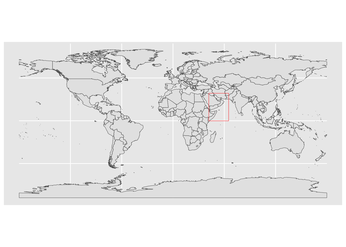

Get occurrence data from robis

We will download data for four sea turtles found in the Arabian sea and save to one file. We will use the occurrence() function in the robis package.

spp <- c("Chelonia mydas", "Caretta caretta", "Eretmochelys imbricata", "Lepidochelys olivacea", "Natator depressus", "Dermochelys coriacea")

obs <- robis::occurrence(spp, startdate = as.Date("2000-01-01"), geometry = wkt_geometry)

This has many columns that we don’t need. We reduced to fewer columns.

cols.to.use <- c("occurrenceID", "scientificName", 
                 "dateIdentified", "eventDate", 
                 "decimalLatitude", "decimalLongitude", "coordinateUncertaintyInMeters",
                 "individualCount","lifeStage", "sex",
                 "bathymetry",  "shoredistance", "sst", "sss")
obs <- obs[,cols.to.use]

We also added a cleaner date with YYYY-MM-DD format.

obs$date <- as.Date(obs$eventDate)

Save our data

Set up the file names

dir_data <- here::here("data")
fil <- here::here("data", "io-sea-turtles.csv")
readr::write_csv(obs, file=fil)

Later we can reload our data as

fil <- here::here("r-tutorials", "data", "io-sea-turtles.csv")
obs <- read.csv(fil)

Clean the data

Select species.

# subset the occurrences to include just those in the water
obs <- obs %>% 
  subset(bathymetry > 0 & shoredistance > 0 & coordinateUncertaintyInMeters < 200)

# seeing how often each species occurs
table(obs$scientificName)


Caretta caretta  Chelonia mydas 
           5141            7060