Earthdata Search and Discovery

Author

Luiz Lopez (NASA Openscapes) and adapted by Eli Holmes (NOAA)

📘 Learning Objectives

How to authenticate with earthaccess

How to use earthaccess to search for data using spatial and temporal filters

How to explore and work with search results

How to plot a single file

Summary

In this example we will use the earthaccess library to search for data collections from NASA Earthdata. earthaccess is a Python library that simplifies data discovery and access to NASA Earth science data by providing an abstraction layer for NASA’s Common Metadata Repository (CMR) API Search API. The library makes searching for data more approachable by using a simpler notation instead of low level HTTP queries. earthaccess takes the trouble out of Earthdata Login authentication, makes search easier, and provides a stream-line way to download or stream search results into an xarray object.

For more on earthaccess visit the earthaccess GitHub page and/or the earthaccess documentation site. Be aware that earthaccess is under active development.

Prerequisites

An Earthdata Login account is required to access data from NASA Earthdata. Please visit https://urs.earthdata.nasa.gov to register and manage your Earthdata Login account. This account is free to create and only takes a moment to set up.

For those not working in the JupyterHub

You will need to create a code cell and run pip install earthaccess.

Get Started

Import Required Packages

import earthaccess 
import xarray as xr

auth = earthaccess.login()
# are we authenticated?
if not auth.authenticated:
    # ask for credentials and persist them in a .netrc file
    auth.login(strategy="interactive", persist=True)

Find a data collection

In NASA Earthdata, a “data collection” refers to a group of related data files, often from a specific satellite or instrument. For this tutorial, we will be search for files (called granules) within specific data collections, so we need to know how to specify a collection. We can specify a collection via a concept_id, doi or short_name. Each of these can be used to search for data or information related to the collection we are interested in. Go through the NASA Earthdata Catalog (0-earthdata-catalog.ipynb) tutorial to learn how to find the identifiers. | Shortname | Collection Concept ID | DOI | | — | — | — | | MUR-JPL-L4-GLOB-v4.1 | C1996881146-POCLOUD | 10.5067/GHGMR-4FJ04 | | AVHRR_OI-NCEI-L4-GLOB-v2.1 | C2036881712-POCLOUD | 10.5067/GHAAO-4BC21 |

Search the collection

We will use the GHRSST Level 4 AVHRR_OI Global Blended Sea Surface Temperature Analysis data from NCEI which has short name AVHRR_OI-NCEI-L4-GLOB-v2.1. We can search via the shortname, concept id or doi.

short_name = 'AVHRR_OI-NCEI-L4-GLOB-v2.1'
results = earthaccess.search_data(
    short_name = short_name,
)
len(results)

concept_id = 'C2036881712-POCLOUD'
results = earthaccess.search_data(
    concept_id = concept_id
)
len(results)

doi = '10.5067/GHAAO-4BC21'
results = earthaccess.search_data(
    doi = doi
)
len(results)

NOTE: Each Earthdata collection has a unique concept_id and doi. This is not the case with short_name. A shortname can be associated with multiple versions of a collection. If multiple versions of a collection are publicaly available, using the short_name parameter with return all versions available. It is advised to use the version parameter in conjunction with the short_name parameter with searching.

Refining the search

We can refine our search by passing more parameters that describe the spatiotemporal domain of our use case. Here, we use the temporal parameter to request a date range and the bounding_box parameter to request granules that intersect with a bounding box.

For our bounding box, we need the xmin, ymin, xmax, ymax and we will assign this to bbox. We will assign our start date and end date to a variable named date_range . We can also specify that we only want cloud hosted data.

date_range = ("2020-01-16", "2020-12-16")
# (xmin=-73.5, ymin=33.5, xmax=-43.5, ymax=43.5)
bbox = (-73.5, 33.5, -43.5, 43.5)

results = earthaccess.search_data(
    concept_id = concept_id,
    cloud_hosted = True,
    temporal = date_range,
    bounding_box = bbox,
)
len(results)

The short_name and concept_id search parameters can be used to request one or multiple collections per request, but the doi parameter can only request a single collection.
> concept_ids = [‘C2723754864-GES_DISC’, ‘C1646609808-NSIDC_ECS’]
Use the cloud_hosted search parameter only to search for data assets available from NASA’s Earthdata Cloud.
There are even more search parameters that can be passed to help refine our search, however those parameters do have to be populated in the CMR record to be leveraged. A non exhaustive list of examples are below:
- day_night_flag = 'day'
- cloud_cover = (0, 10)

Working with `earthaccess` returns

Following the search for data, you’ll likely take one of two pathways with those results. You may choose to download the assets that have been returned to you or you may choose to continue working with the search results within the Python environment.

type(results[0])

earthaccess.results.DataGranule

results[0]

Data: 20200115120000-NCEI-L4_GHRSST-SSTblend-AVHRR_OI-GLOB-v02.0-fv02.1.nc

Size: 0.99 MB

Cloud Hosted: True

Download `earthaccess` results

In some cases you may want to download your assets. earthaccess makes downloading the data from the search results very easy using the earthaccess.download() function.

downloaded_files = earthaccess.download( results[0:9], local_path=‘../data’, )

earthaccess does a lot of heavy lifting for us. It identifies the downloadable links, passes our Earthdata Login credentials, and saves the files with the proper names.

Stream data to memory rather than downloading

Alternatively we can work with the metadata without downloading and only load the data into memory (or download) when we need to compute with it or plot it.

The data_links() methods gets us the url to the data. The data_links() method can also be used to get the s3 URI when we want to perform direct s3 access of the data in the cloud. To get the s3 URI, pass access = 'direct' to the method. Note, for NASA data, you need to be in AWS us-west-2 for direct access to work.

results[0].data_links()

['https://archive.podaac.earthdata.nasa.gov/podaac-ops-cumulus-protected/AVHRR_OI-NCEI-L4-GLOB-v2.1/20200115120000-NCEI-L4_GHRSST-SSTblend-AVHRR_OI-GLOB-v02.0-fv02.1.nc']

We can pass or read the data url into libraries like xarray, rioxarray, or gdal, but we would need to deal with the authentication. earthaccess has a built-in module for easily reading these data links in and takes care of authentication for us.

We use earthaccess’s open() method make a connection the cloud resource so we can work with the files. To get the first file, we use results[0:1].

fileset = earthaccess.open(results[0:1])

fileset

[<File-like object S3FileSystem, podaac-ops-cumulus-protected/AVHRR_OI-NCEI-L4-GLOB-v2.1/20200115120000-NCEI-L4_GHRSST-SSTblend-AVHRR_OI-GLOB-v02.0-fv02.1.nc>]

ds = xr.open_dataset(fileset[0])
ds

We can plot this object.

ds['analysed_sst'].plot();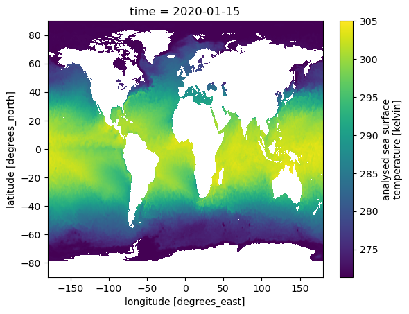

Conclusion

You have worked with remote-sensing data in the cloud and plotted a single file.

Next we will learn to subset the data so we can work with bigger datasets in the cloud without downloading the whole dataset.