Extract data within a boundary

Author

NOAA CoastWatch with modifications to use earthaccess by Eli Holmes

📘 Learning Objectives

How to trim satellite data to specific bounding coordinates

How to apply shapefiles as masks to satellite data

How to compute and plot means within the shapefiles

Summary

This example is adapted from the NOAA CoastWatch Tutorial Github repository.. It shows you how to get a time series of daily SST within a region defined by a shapefile.

For those not working in the JupyterHub

Create a code cell and run pip install earthaccess, pip install regionmask, pip install cartopy

Datasets used

GHRSST Level 4 AVHRR_OI Global Blended Sea Surface Temperature Analysis (GDS2) from NCEI
This NOAA blended SST is a moderate resolution satellite-based gap-free sea surface temperature (SST) product. We will use the daily data. https://cmr.earthdata.nasa.gov/search/concepts/C2036881712-POCLOUD.html

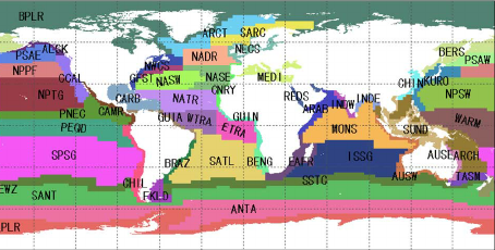
Longhurst Marine Provinces
The dataset represents the division of the world oceans into provinces as defined by Longhurst (1995; 1998; 2006). This division has been based on the prevailing role of physical forcing as a regulator of phytoplankton distribution.

The Longhurst Marine Provinces dataset is available online (https://www.marineregions.org/downloads.php) and within the shapes folder associated with this repository. For this exercise we will use the Gulf Stream province (ProvCode: GFST)

Import packages and authenticate

import earthaccess 
from pprint import pprint
import xarray as xr
import geopandas as gpd

import regionmask
import os
import matplotlib.pyplot as plt
import cartopy.crs as ccrs
import cartopy.feature as cfeature
from cartopy.mpl.ticker import LongitudeFormatter, LatitudeFormatter

import warnings
warnings.filterwarnings("ignore")

os.environ["HOME"] = "/home/jovyan"

auth = earthaccess.login()
# are we authenticated?
if not auth.authenticated:
    # ask for credentials and persist them in a .netrc file
    auth.login(strategy="interactive", persist=True)

Load the Longhurst Provinces shape files into a geopandas dataframe

#shape_path = '../resources/longhurst_v4_2010/Longhurst_world_v4_2010.shp'
shape_path = os.path.join('..',
                          'resources',
                          'longhurst_v4_2010',
                          'Longhurst_world_v4_2010.shp'
                          )
shapefiles = gpd.read_file(shape_path)
shapefiles.head(8)

	ProvCode	ProvDescr	geometry
0	BPLR	Polar - Boreal Polar Province (POLR)	MULTIPOLYGON (((-161.18426 63.5, -161.5 63.5, ...
1	ARCT	Polar - Atlantic Arctic Province	MULTIPOLYGON (((-21.51305 64.64409, -21.55945 ...
2	SARC	Polar - Atlantic Subarctic Province	MULTIPOLYGON (((11.26472 63.96082, 11.09548 63...
3	NADR	Westerlies - N. Atlantic Drift Province (WWDR)	POLYGON ((-11.5 57.5, -11.5 56.5, -11.5 55.5, ...
4	GFST	Westerlies - Gulf Stream Province	POLYGON ((-43.5 43.5, -43.5 42.5, -43.5 41.5, ...
5	NASW	Westerlies - N. Atlantic Subtropical Gyral Pro...	POLYGON ((-39.5 25.5, -40.5 25.5, -41.5 25.5, ...
6	NATR	Trades - N. Atlantic Tropical Gyral Province (...	MULTIPOLYGON (((-72.34673 18.53597, -72.36877 ...
7	WTRA	Trades - Western Tropical Atlantic Province	POLYGON ((-19.5 -6.5, -20.5 -6.5, -21.5 -6.5, ...

Isolate the Gulf Stream Province

The Gulf Stream Province can be isolated using its ProvCode (GFST)

ProvCode = "GFST"

# Locate the row with the ProvCode code
gulf_stream = shapefiles.loc[shapefiles["ProvCode"] == ProvCode]
gulf_stream

	ProvCode	ProvDescr	geometry
4	GFST	Westerlies - Gulf Stream Province	POLYGON ((-43.5 43.5, -43.5 42.5, -43.5 41.5, ...

Find the coordinates of the bounding box

The bounding box is the smallest rectangle that will completely enclose the province.
We will use the bounding box coordinates to subset the satellite data

gs_bnds = gulf_stream.bounds
gs_bnds

	minx	miny	maxx	maxy
4	-73.5	33.5	-43.5	43.5

Search and access NASA Earthdata with the Collection Concept ID

Shortname	Collection Concept ID	DOI
AVHRR_OI-NCEI-L4-GLOB-v2.1	C2036881712-POCLOUD	10.5067/GHAAO-4BC21

# Search Dataset Unique ID
collection_id = 'C2036881712-POCLOUD'
results = earthaccess.search_data(
    concept_id = collection_id,
)

# Define date range and bounding box and search
date_range = ("2020-01-16", "2020-3-16")
# (xmin=-73.5, ymin=33.5, xmax=-43.5, ymax=43.5)
bbox = (gs_bnds.minx, gs_bnds.miny, gs_bnds.maxx, gs_bnds.maxy)

# Get results based on date range and bbox
results = earthaccess.search_data(
    concept_id = collection_id,
    cloud_hosted = True,
    temporal = date_range,
    bounding_box = bbox,
)

#Examine results

item = results[0]
#type(item)
#item.keys()
item['umm']

{'TemporalExtent': {'RangeDateTime': {'EndingDateTime': '2020-01-16T00:00:00.000Z',
   'BeginningDateTime': '2020-01-15T00:00:00.000Z'}},
 'MetadataSpecification': {'URL': 'https://cdn.earthdata.nasa.gov/umm/granule/v1.6.6',
  'Name': 'UMM-G',
  'Version': '1.6.6'},
 'GranuleUR': '20200115120000-NCEI-L4_GHRSST-SSTblend-AVHRR_OI-GLOB-v02.0-fv02.1',
 'ProviderDates': [{'Type': 'Insert', 'Date': '2021-05-11T17:17:16.602Z'},
  {'Type': 'Update', 'Date': '2021-05-11T17:17:16.603Z'}],
 'SpatialExtent': {'HorizontalSpatialDomain': {'Geometry': {'BoundingRectangles': [{'WestBoundingCoordinate': -179.875,
      'SouthBoundingCoordinate': -89.875,
      'EastBoundingCoordinate': 179.875,
      'NorthBoundingCoordinate': 89.875}]}}},
 'DataGranule': {'ArchiveAndDistributionInformation': [{'SizeUnit': 'MB',
    'Size': 9.72747802734375e-05,
    'Checksum': {'Value': 'f7f272ac28fd5563da4a03bc9c74a9c2',
     'Algorithm': 'MD5'},
    'SizeInBytes': 102,
    'Name': '20200115120000-NCEI-L4_GHRSST-SSTblend-AVHRR_OI-GLOB-v02.0-fv02.1.nc.md5'},
   {'SizeUnit': 'MB',
    'Size': 0.9890298843383789,
    'Checksum': {'Value': '779e063e913ff1df721b252bbc4eb3b9',
     'Algorithm': 'MD5'},
    'SizeInBytes': 1037073,
    'Name': '20200115120000-NCEI-L4_GHRSST-SSTblend-AVHRR_OI-GLOB-v02.0-fv02.1.nc'}],
  'DayNightFlag': 'Unspecified',
  'ProductionDateTime': '2020-02-11T00:00:00.000Z'},
 'CollectionReference': {'Version': '2.1',
  'ShortName': 'AVHRR_OI-NCEI-L4-GLOB-v2.1'},
 'RelatedUrls': [{'URL': 's3://podaac-ops-cumulus-protected/AVHRR_OI-NCEI-L4-GLOB-v2.1/20200115120000-NCEI-L4_GHRSST-SSTblend-AVHRR_OI-GLOB-v02.0-fv02.1.nc',
   'Type': 'GET DATA VIA DIRECT ACCESS',
   'Description': 'This link provides direct download access via S3 to the granule.'},
  {'URL': 'https://archive.podaac.earthdata.nasa.gov/podaac-ops-cumulus-public/AVHRR_OI-NCEI-L4-GLOB-v2.1/20200115120000-NCEI-L4_GHRSST-SSTblend-AVHRR_OI-GLOB-v02.0-fv02.1.nc.md5',
   'Description': 'Download 20200115120000-NCEI-L4_GHRSST-SSTblend-AVHRR_OI-GLOB-v02.0-fv02.1.nc.md5',
   'Type': 'EXTENDED METADATA'},
  {'URL': 'https://archive.podaac.earthdata.nasa.gov/podaac-ops-cumulus-protected/AVHRR_OI-NCEI-L4-GLOB-v2.1/20200115120000-NCEI-L4_GHRSST-SSTblend-AVHRR_OI-GLOB-v02.0-fv02.1.nc',
   'Description': 'Download 20200115120000-NCEI-L4_GHRSST-SSTblend-AVHRR_OI-GLOB-v02.0-fv02.1.nc',
   'Type': 'GET DATA'},
  {'URL': 'https://archive.podaac.earthdata.nasa.gov/s3credentials',
   'Description': 'api endpoint to retrieve temporary credentials valid for same-region direct s3 access',
   'Type': 'VIEW RELATED INFORMATION'},
  {'URL': 'https://opendap.earthdata.nasa.gov/providers/POCLOUD/collections/GHRSST%20Level%204%20AVHRR_OI%20Global%20Blended%20Sea%20Surface%20Temperature%20Analysis%20(GDS2)%20from%20NCEI/granules/20200115120000-NCEI-L4_GHRSST-SSTblend-AVHRR_OI-GLOB-v02.0-fv02.1',
   'Type': 'USE SERVICE API',
   'Subtype': 'OPENDAP DATA',
   'Description': 'OPeNDAP request URL'}]}

# Get the first 30 files
fileset = earthaccess.open(results[1:30])

Load the satellite data

# Load data; takes awhile
ds = xr.open_mfdataset(fileset, chunks = {})

# Get SST data 
ds_subset = ds['analysed_sst']

Visualize the unmasked data on a map

The map shows the full extent of the bounding box

plt.figure(figsize=(14, 10))

# Label axes of a Plate Carree projection with a central longitude of 180:
ax1 = plt.subplot(211, projection=ccrs.PlateCarree(central_longitude=180))

# Use the lon and lat ranges to set the extent of the map
# the 120, 260 lon range will show the whole Pacific
# the 15, 55 lat range with capture the range of the data
ax1.set_extent([260, 350, 15, 55], ccrs.PlateCarree())

# set the tick marks to be slightly inside the map extents

# add feature to the map
ax1.add_feature(cfeature.LAND, facecolor='0.6')
ax1.coastlines()

# format the lat and lon axis labels
lon_formatter = LongitudeFormatter(zero_direction_label=True)
lat_formatter = LatitudeFormatter()
ax1.xaxis.set_major_formatter(lon_formatter)
ax1.yaxis.set_major_formatter(lat_formatter)

sst_cm = ds_subset[0].plot.pcolormesh(ax=ax1, transform=ccrs.PlateCarree(), cmap='jet')
plt.title('Satellite Data Before Masking')

Text(0.5, 1.0, 'Satellite Data Before Masking')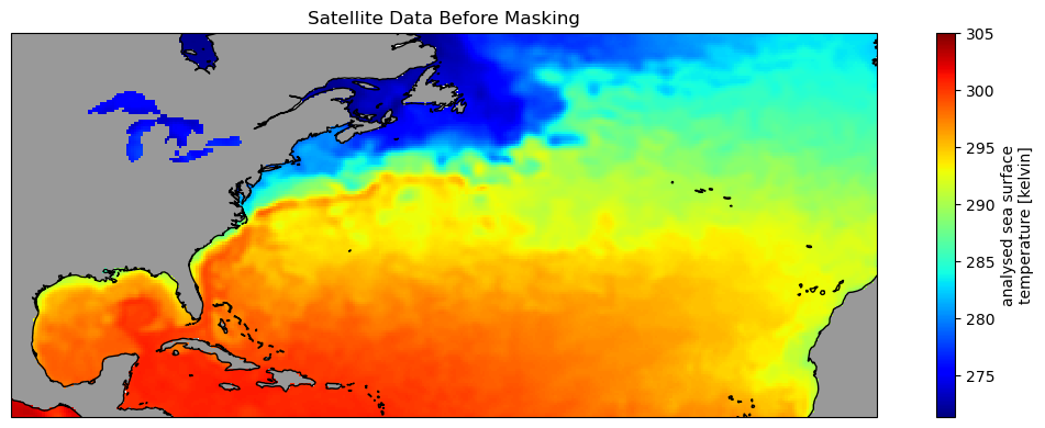

Create the region from the shape file

The plot shows the shape of the region and its placement along the US East Coast.

region = regionmask.from_geopandas(gulf_stream)
region.plot()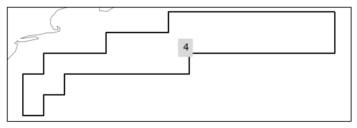

Mask the satellite data

# Create the mask
mask = region.mask(ds_subset.lon, ds_subset.lat)

# Apply mask the the satellite data
masked_ds = ds_subset.where(mask == region.numbers[0])

Visualize the masked data on a map

These data have been trimmed to contain only values within the Gulf Stream Province

plt.figure(figsize=(14, 10))

# Label axes of a Plate Carree projection with a central longitude of 180:
ax1 = plt.subplot(211, projection=ccrs.PlateCarree(central_longitude=180))

# Use the lon and lat ranges to set the extent of the map
# the 120, 260 lon range will show the whole Pacific
# the 15, 55 lat range with capture the range of the data
ax1.set_extent([260, 350, 15, 55], ccrs.PlateCarree())

# add feature to the map
ax1.add_feature(cfeature.LAND, facecolor='0.6')
ax1.coastlines()

masked_ds[0].plot.pcolormesh(ax=ax1,
                             transform=ccrs.PlateCarree(),
                             cmap='jet')

plt.title('Satellite Data After Masking for Longhurst GFST');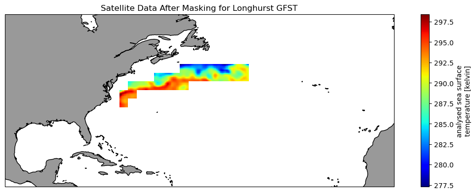

Calculate the mean temperature over all timesteps

# Calculate mean over all time steps
sst_mean_grid = masked_ds.mean(dim='time')

# Map the SST mean
sst_mean_grid.plot()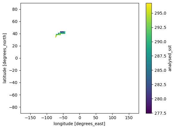

Calculate the mean temperature over all grids (lat, lon)

# Calculate mean over all grids
sst_mean_time = masked_ds.mean(dim=['lat', 'lon'])

# Plot the SST mean
plt.figure(figsize=(10, 5)) 
plt.plot_date(sst_mean_time.time,
              sst_mean_time, 
              'o', markersize=8, 
              label='gulf stream', c='black', 
              linestyle='-', linewidth=2) 

plt.title('Gulf Stream Province Daily Mean Temperature 2020')
plt.ylabel('SST (degrees C)') 
plt.xlabel('Dates')
plt.legend()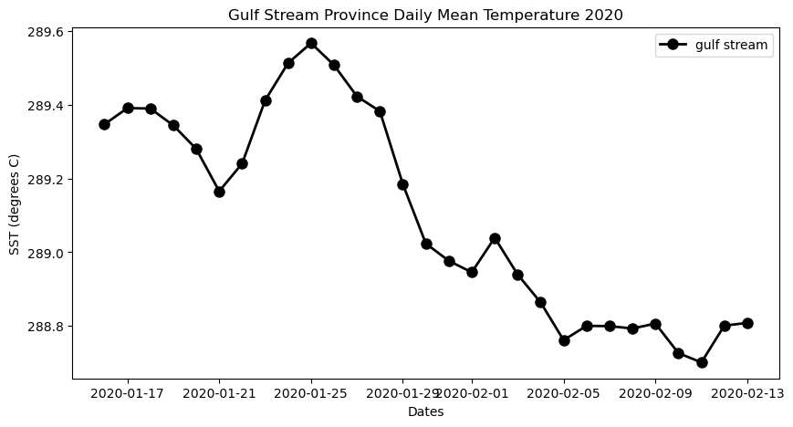

References

AVHRR SST Data
NASA Earthdata catalog
To explore a full range of tutorials on accessing and utilizing oceanographic satellite data, visit the NOAA CoastWatch Tutorial Github repository.. These tutorials use ERDDAP servers but code for minulating the data cubes is the same as that use with data from NASA Earthdata.
Sources for marine shape files: https://www.marineregions.org/downloads.php