PACE Level 2 plots for Rrs and AVW

Figures

Overview

The figures were generated from Level 2 products.

The PACE Level-2 OCI (ocean color instrument) data is available on an NASA EarthData. Search using the instrument filter “OCI” and processing level 2 filter https://search.earthdata.nasa.gov/search?fi=OCI&fl=2%2B-%2BGeophys.%2BVariables%252C%2BSensor%2BCoordinates and you will see 16 data collections.

The Level 2 netcdf files are grouped with the geophysical data, lat/lon, and wavelength data in different groups.

Data collection used

• date: 2024-05-13
• spatial bin: T171853
• spatial extent: lat=[38.0,42.5]; lon=[-75.5,-69.0];

PACE OCI Level-2 Regional Apparent Optical Properties Data, version 3.0

• https://cmr.earthdata.nasa.gov/search/concepts/C3385049983-OB_CLOUD.html
• remote sensing reflectance and avw
• short name: PACE_OCI_L2_AOP
• filename: PACE_OCI.20240513T171853.L2.OC_AOP.V3_0_0.nc

PACE OCI Level-2 Regional Ocean Biogeochemical Properties Data, version 3.0

• https://cmr.earthdata.nasa.gov/search/concepts/C3385050002-OB_CLOUD.html
• variables include carbon_phyto, chlor_a, poc
• short name: PACE_OCI_L2_BGC

Prerequisites

You need to have an EarthData Login username and password. Go here to get one https://urs.earthdata.nasa.gov/

I assume you have a .netrc file at ~ (home). ~/.netrc should look just like this with your username and password. Create that file if needed. You don’t need to create it if you don’t have this file. The earthaccess.login(persist=True) line will ask for your username and password and create the .netrc file for you.

machine urs.earthdata.nasa.gov
        login yourusername
        password yourpassword

For those not working in the JupyterHub

Uncomment this and run the cell:

# pip install earthaccess

Rrs figures

Get data

%%time
# Authenticate to NASA
import earthaccess
auth = earthaccess.login(strategy="interactive", persist=True)
    
# (xmin=-73.5, ymin=33.5, xmax=-43.5, ymax=43.5)
bbox = (-75.5, 38.0, -69.0, 42.5)
import earthaccess
results = earthaccess.search_data(
    short_name = "PACE_OCI_L2_AOP",
    temporal = ("2024-05-13", "2024-05-13"),
    bounding_box = bbox
)
fileset = earthaccess.open(results);

CPU times: user 475 ms, sys: 77 ms, total: 552 ms
Wall time: 8 s

Examine the groups

import h5netcdf
with h5netcdf.File(fileset[0]) as file:
    groups = list(file)
groups

['sensor_band_parameters',
 'scan_line_attributes',
 'geophysical_data',
 'navigation_data',
 'processing_control']

Process data and subset

%%time
import xarray as xr
ds = xr.open_dataset(fileset[0], group="geophysical_data")

# Add coords
# Add coords
nav = xr.open_dataset(fileset[0], group="navigation_data")
nav = nav.set_coords(("longitude", "latitude"))
wave = xr.open_dataset(fileset[0], group="sensor_band_parameters")
wave = wave.set_coords(("wavelength_3d"))
dataset = xr.merge((ds["Rrs"], nav.coords, wave.coords))

# Subset
rrs_box = dataset.where(
    (
        (dataset["latitude"] > 38.0)
        & (dataset["latitude"] < 42.5)
        & (dataset["longitude"] > -75.5)
        & (dataset["longitude"] < -69.0)
    ),
    drop = True
)

CPU times: user 12.6 s, sys: 6.03 s, total: 18.6 s
Wall time: 54.7 s

Make plots

# make single plot
import matplotlib.pyplot as plt

rrs = rrs_box["Rrs"].sel(wavelength_3d = 380)
plot = rrs.plot(x="longitude", y="latitude", cmap="jet", vmin=0, vmax=0.005)

# Set x and y limits
plot.axes.set_xlim(-75.5, -69.0)
plot.axes.set_ylim(38.0, 42.5)

# Customize colorbar label
wave_string = "380"  # or str(wavelength) if dynamic
plot.colorbar.set_label(f"Rrs {wave_string} (sr⁻¹)", fontsize=16, fontweight="bold")

plt.show()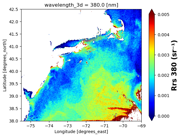

import matplotlib.pyplot as plt
import matplotlib.colors as colors

# List of wavelengths to plot
wavelengths = [380, 442, 490, 550, 670, 588]

# Create figure and axes
fig, axes = plt.subplots(3, 2, figsize=(12, 12), constrained_layout=True)
axes = axes.flatten()

# Loop through wavelengths and plot
for i, wl in enumerate(wavelengths):
    ax = axes[i]
    
    # Extract Rrs and mask zeros (for log or safety)
    rrs = rrs_box["Rrs"].sel(wavelength_3d=wl)
    
    # Plot onto the provided axis
    img = rrs.plot(
        ax=ax,
        x="longitude",
        y="latitude",
        cmap="jet",
        vmin=0,
        vmax=0.005,
        add_colorbar=False  # We'll add our own
    )
    
    # Set limits
    ax.set_xlim(-75.5, -69.0)
    ax.set_ylim(38.0, 42.5)
    
    # Add colorbar
    cbar = fig.colorbar(img, ax=ax, orientation="vertical", shrink=0.8)
    cbar.set_label(f"Rrs {wl} (sr⁻¹)", fontsize=12, fontweight="bold")
    
    # Optional: title or annotation
    ax.set_title(f"Wavelength {wl} nm")

# Turn off unused axes (if any)
for j in range(len(wavelengths), len(axes)):
    fig.delaxes(axes[j])

plt.show()

AVW figures

Get and set up data

%%time
# Authenticate to NASA
import earthaccess
auth = earthaccess.login(strategy="interactive", persist=True)
    
# (xmin=-73.5, ymin=33.5, xmax=-43.5, ymax=43.5)
bbox = (-75.5, 38.0, -69.0, 42.5)
import earthaccess
results = earthaccess.search_data(
    short_name = "PACE_OCI_L2_AOP",
    temporal = ("2024-05-13", "2024-05-13"),
    bounding_box = bbox
)
fileset = earthaccess.open(results);

# load data
import xarray as xr
ds = xr.open_dataset(fileset[0], group="geophysical_data")

# Add coords
# Add coords
nav = xr.open_dataset(fileset[0], group="navigation_data")
nav = nav.set_coords(("longitude", "latitude"))
wave = xr.open_dataset(fileset[0], group="sensor_band_parameters")
wave = wave.set_coords(("wavelength_3d"))
dataset = xr.merge((ds["avw"], nav.coords, wave.coords))

# Subset
avw_box = dataset.where(
    (
        (dataset["latitude"] > 38.0)
        & (dataset["latitude"] < 42.5)
        & (dataset["longitude"] > -75.5)
        & (dataset["longitude"] < -69.0)
    ),
    drop = True
)

CPU times: user 5.44 s, sys: 3.05 s, total: 8.49 s
Wall time: 36.9 s

# make one plot
import matplotlib.pyplot as plt

plot = avw_box["avw"].plot(x="longitude", y="latitude", cmap="jet", vmin=450, vmax=580)

# Set x and y limits
plot.axes.set_xlim(-75.5, -69.0)
plot.axes.set_ylim(38.0, 42.5)

# Customize colorbar label
plot.colorbar.set_label("AVW (nm)", fontsize=16, fontweight="bold")

plt.show()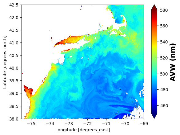

Chlorophyll figures

Level 2 Chlorophyll is in the Ocean Biogeochemical Properties product.

%%time
# Authenticate to NASA
import earthaccess
auth = earthaccess.login(strategy="interactive", persist=True)
    
# (xmin=-73.5, ymin=33.5, xmax=-43.5, ymax=43.5)
bbox = (-75.5, 38.0, -69.0, 42.5)
import earthaccess
results = earthaccess.search_data(
    short_name = "PACE_OCI_L2_BGC",
    temporal = ("2024-05-13", "2024-05-13"),
    bounding_box = bbox
)
fileset = earthaccess.open(results);

CPU times: user 474 ms, sys: 80.9 ms, total: 555 ms
Wall time: 11.4 s

Examine groups

import h5netcdf
with h5netcdf.File(fileset[0]) as file:
    groups = list(file)
groups

['sensor_band_parameters',
 'scan_line_attributes',
 'geophysical_data',
 'navigation_data',
 'processing_control']

import xarray as xr
ds = xr.open_dataset(fileset[0], group="geophysical_data")
ds

<xarray.Dataset> Size: 52MB
Dimensions:           (number_of_lines: 1709, pixels_per_line: 1272)
Dimensions without coordinates: number_of_lines, pixels_per_line
Data variables:
    chlor_a           (number_of_lines, pixels_per_line) float32 9MB ...
    carbon_phyto      (number_of_lines, pixels_per_line) float32 9MB ...
    poc               (number_of_lines, pixels_per_line) float32 9MB ...
    chlor_a_unc       (number_of_lines, pixels_per_line) float32 9MB ...
    carbon_phyto_unc  (number_of_lines, pixels_per_line) float32 9MB ...
    l2_flags          (number_of_lines, pixels_per_line) int32 9MB ...

xarray.Dataset

• Dimensions:
  • number_of_lines: 1709
  • pixels_per_line: 1272
• Coordinates: (0)
• Data variables: (6)
  • chlor_a
    (number_of_lines, pixels_per_line)
    float32
    ...

    long_name :

    Chlorophyll Concentration, OCI Algorithm

    units :

    mg m^-3

    standard_name :

    mass_concentration_of_chlorophyll_in_sea_water

    valid_min :

    0.001

    valid_max :

    100.0

    reference :

    Hu, C., Lee Z., and Franz, B.A. (2012). Chlorophyll-a algorithms for oligotrophic oceans: A novel approach based on three-band reflectance difference, J. Geophys. Res., 117, C01011, doi:10.1029/2011JC007395.

    [2173848 values with dtype=float32]

  • carbon_phyto
    (number_of_lines, pixels_per_line)
    float32
    ...

    long_name :

    Phytoplankton Carbon

    units :

    mg m^-3

    valid_min :

    0.0

    valid_max :

    1000.0

    reference :

    Graff, J.R., Westberry, T.K., Milligan, A.J., Brown, M.B., Dall'Olmo, G., Dongen-Vogels, V.v., Reifel, K.M., and Behrenfeld, M.J. (2015). Analytical phytoplankton carbon measurements spanning diverse ecosystems. Deep Sea Research Part I: Oceanographic Research Papers, 102, 16-25

    [2173848 values with dtype=float32]

  • poc
    (number_of_lines, pixels_per_line)
    float32
    ...

    long_name :

    Particulate Organic Carbon, D. Stramski, 2022 (hybrid version)

    units :

    mg m^-3

    valid_min :

    -32000

    valid_max :

    -22000

    reference :

    Stramski, D., et al. "Ocean color algorithms to estimate the concentration of particulate organic carbon in surface waters of the global ocean in support of a long-term data record from multiple satellite missions." Remote Sensing of Environment 269 (2022)

    [2173848 values with dtype=float32]

  • chlor_a_unc
    (number_of_lines, pixels_per_line)
    float32
    ...

    long_name :

    Uncertainty in chlorophyll a concentration

    units :

    mg m^-3

    standard_name :

    chlorophyll_concentration_in_sea_water standard_error

    valid_min :

    0.001

    valid_max :

    100.0

    [2173848 values with dtype=float32]

  • carbon_phyto_unc
    (number_of_lines, pixels_per_line)
    float32
    ...

    long_name :

    Phytoplankton Carbon standard uncertainty

    units :

    mg m^-3

    valid_min :

    0.0

    valid_max :

    1000.0

    reference :

    Graff, J.R., Westberry, T.K., Milligan, A.J., Brown, M.B., Dall'Olmo, G., Dongen-Vogels, V.v., Reifel, K.M., and Behrenfeld, M.J. (2015). Analytical phytoplankton carbon measurements spanning diverse ecosystems. Deep Sea Research Part I: Oceanographic Research Papers, 102, 16-25

    [2173848 values with dtype=float32]

  • l2_flags
    (number_of_lines, pixels_per_line)
    int32
    ...

    long_name :

    Level-2 Processing Flags

    valid_min :

    -2147483648

    valid_max :

    2147483647

    flag_masks :

    [ 1 2 4 8 16 32 64 128 256 512 1024 2048 4096 8192 16384 32768 65536 131072 262144 524288 1048576 2097152 4194304 8388608 16777216 33554432 67108864 134217728 268435456 536870912 1073741824 -2147483648]

    flag_meanings :

    ATMFAIL LAND PRODWARN HIGLINT HILT HISATZEN COASTZ SPARE STRAYLIGHT CLDICE COCCOLITH TURBIDW HISOLZEN SPARE LOWLW CHLFAIL NAVWARN ABSAER SPARE MAXAERITER MODGLINT CHLWARN ATMWARN SPARE SEAICE NAVFAIL FILTER SPARE BOWTIEDEL HIPOL PRODFAIL SPARE

    [2173848 values with dtype=int32]

• Indexes: (0)
• Attributes: (0)

Process data and subset

%%time
import xarray as xr
ds = xr.open_dataset(fileset[0], group="geophysical_data")

# Add coords
# Add coords
nav = xr.open_dataset(fileset[0], group="navigation_data")
nav = nav.set_coords(("longitude", "latitude"))
dataset = xr.merge((ds["chlor_a"], nav.coords))

# Subset
chla_box = dataset.where(
    (
        (dataset["latitude"] > 38.0)
        & (dataset["latitude"] < 42.5)
        & (dataset["longitude"] > -75.5)
        & (dataset["longitude"] < -69.0)
    ),
    drop = True
)

CPU times: user 276 ms, sys: 12.3 ms, total: 288 ms
Wall time: 287 ms

import matplotlib.pyplot as plt
from matplotlib.colors import LogNorm

chl = chla_box["chlor_a"].where(chla_box["chlor_a"] > 0)

plot = plt.pcolormesh(
    chla_box["longitude"], chla_box["latitude"], chl,
    cmap="jet", norm=LogNorm(vmin=1e-2, vmax=1e1), shading="auto"
)
cbar = plt.colorbar(plot)
cbar.set_label("Chlorophyll-a (mg m⁻³)", fontsize=16, fontweight="bold")

plt.xlim(-75.5, -69.0)
plt.ylim(38.0, 42.5)
plt.xlabel("Longitude")
plt.ylabel("Latitude")
plt.title("Chlorophyll-a (Log Scale)")

plt.show()

Carbon phyto

%%time
import xarray as xr
ds = xr.open_dataset(fileset[0], group="geophysical_data")

# Add coords
# Add coords
nav = xr.open_dataset(fileset[0], group="navigation_data")
nav = nav.set_coords(("longitude", "latitude"))
dataset = xr.merge((ds["carbon_phyto"], nav.coords))

# Subset
carbon_phyto_box = dataset.where(
    (
        (dataset["latitude"] > 38.0)
        & (dataset["latitude"] < 42.5)
        & (dataset["longitude"] > -75.5)
        & (dataset["longitude"] < -69.0)
    ),
    drop = True
)

CPU times: user 277 ms, sys: 7.89 ms, total: 285 ms
Wall time: 284 ms

import matplotlib.pyplot as plt
from matplotlib.colors import LogNorm

cp = carbon_phyto_box["carbon_phyto"].where(carbon_phyto_box["carbon_phyto"] > 0)

plot = plt.pcolormesh(
    carbon_phyto_box["longitude"], carbon_phyto_box["latitude"], cp,
    cmap="jet", norm=LogNorm(vmin=1e1, vmax=500), shading="auto"
)
cbar = plt.colorbar(plot)
cbar.set_label("Phytoplankton Carbon (mg m⁻³)", fontsize=16, fontweight="bold")

plt.xlim(-75.5, -69.0)
plt.ylim(38.0, 42.5)
plt.xlabel("Longitude")
plt.ylabel("Latitude")
plt.title("Phytoplankton Carbon (Log Scale)")

plt.show()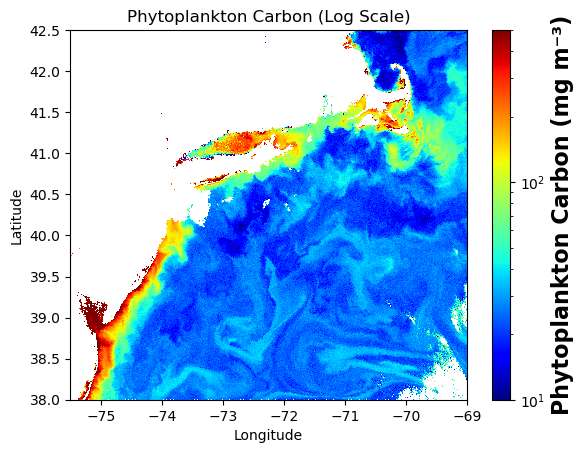

cp.max()

<xarray.DataArray 'carbon_phyto' ()> Size: 4B
array(1739.7222, dtype=float32)

xarray.DataArray

'carbon_phyto'

• 1.74e+03

  array(1739.7222, dtype=float32)

• Coordinates: (0)
• Indexes: (0)
• Attributes: (0)