📘 Learning Objectives
Show how to work with the earthaccess package for PACE data
Create a NASA EDL session for authentication
Load single files with xarray.open_dataset
Load multiple files with xarray.open_mfdataset
Overview
The PACE Level-3 (gridded) OCI (ocean color instrument) data is available on an NASA EarthData. Search using the instrument filter “OCI” and processing level filter “Gridded Observations” https://search.earthdata.nasa.gov/search?fi=OCI&fl=3%2B-%2BGridded%2BObservations and you will see 45+ data collections. In this tutorial, we will look at the Apparent Visible Wavelength (AVW) product.
The collection information page is here: PACE OCI Level-3 Global Mapped Apparent Visible Wavelength (AVW) Data, version 3.0 . The concept id for this dataset is “C3385050418-OB_CLOUD” and the short name is “PACE_OCI_L3M_AVW”.
Prerequisites
You need to have an EarthData Login username and password. Go here to get one https://urs.earthdata.nasa.gov/
I assume you have a .netrc file at ~ (home). ~/.netrc should look just like this with your username and password. Create that file if needed. You don’t need to create it if you don’t have this file. The earthaccess.login(persist=True) line will ask for your username and password and create the .netrc file for you.
machine urs.earthdata.nasa.gov
        login yourusername
        password yourpassword
For those not working in the JupyterHub
Uncomment this and run the cell:
# pip install earthaccess
Create a NASA EDL authenticated session
Authenticate with earthaccess.login().Authenticate with earthaccess.login(). You will need your EarthData Login username and password for this step. Get one here https://urs.earthdata.nasa.gov/ .
import earthaccess= earthaccess.login()# are we authenticated? if not auth.authenticated:# ask for credentials and persist them in a .netrc file = "interactive" , persist= True )
Monthly data
I poked around on the files on search.earthdata so I know what the files look like.
import earthaccess= earthaccess.search_data(= "PACE_OCI_L3M_AVW" ,= ("2024-03-01" , "2024-10-31" ),= "*.MO.*.0p1deg.*" len (results_mo)
# Create a fileset = earthaccess.open (results_mo);
# let's load just one month import xarray as xr= xr.open_dataset(fileset[0 ])
<xarray.Dataset> Size: 26MB
Dimensions:  (lat: 1800, lon: 3600, rgb: 3, eightbitcolor: 256)
Coordinates:
  * lat      (lat) float32 7kB 89.95 89.85 89.75 89.65 ... -89.75 -89.85 -89.95
  * lon      (lon) float32 14kB -179.9 -179.9 -179.8 ... 179.8 179.9 180.0
Dimensions without coordinates: rgb, eightbitcolor
Data variables:
    avw      (lat, lon) float32 26MB ...
    palette  (rgb, eightbitcolor) uint8 768B ...
Attributes: (12/62)
    product_name:                      PACE_OCI.20240301_20240331.L3m.MO.AVW....
    instrument:                        OCI
    title:                             OCI Level-3 Standard Mapped Image
    project:                           Ocean Biology Processing Group (NASA/G...
    platform:                          PACE
    source:                            satellite observations from OCI-PACE
    ...                                ...
    cdm_data_type:                     grid
    identifier_product_doi_authority:  http://dx.doi.org
    identifier_product_doi:            10.5067/PACE/OCI/L3M/AVW/3.0
    data_bins:                         3016790
    data_minimum:                      399.99997
data_maximum: 700.00006 Dimensions: lat : 1800lon : 3600rgb : 3eightbitcolor : 256
Coordinates: (2)
Data variables: (2)
avw
(lat, lon)
float32
...
long_name : Apparent Visible Wavelength units : nm valid_min : 400.0 valid_max : 700.0 reference : Vandermeulen, R. A., Mannino, A., Craig, S.E., Werdell, P.J., 2020: 150 shades of green: Using the full spectrum of remote sensing reflectance to elucidate color shifts in the ocean, Remote Sensing of Environment, 247, 111900, https://doi.org/10.1016/j.rse.2020.111900, https://doi.org/10.5067/KAROCHG01RYJ display_scale : linear display_min : 450.0 display_max : 575.0 [6480000 values with dtype=float32] palette
(rgb, eightbitcolor)
uint8
...
[768 values with dtype=uint8] Indexes: (2)
PandasIndex
PandasIndex(Index([ 89.94999694824219,   89.8499984741211,              89.75,
         89.6500015258789,  89.55000305175781,  89.44999694824219,
         89.3499984741211,              89.25,   89.1500015258789,
        89.05000305175781,
       ...
       -89.05000305175781,  -89.1500015258789,             -89.25,
       -89.35000610351562, -89.45000457763672, -89.55000305175781,
        -89.6500015258789,             -89.75, -89.85000610351562,
       -89.95000457763672],
dtype='float32', name='lat', length=1800)) PandasIndex
PandasIndex(Index([ -179.9499969482422, -179.85000610351562,             -179.75,
       -179.64999389648438,  -179.5500030517578,  -179.4499969482422,
       -179.35000610351562,             -179.25, -179.14999389648438,
        -179.0500030517578,
       ...
         179.0500030517578,  179.15000915527344,              179.25,
        179.35000610351562,  179.45001220703125,   179.5500030517578,
        179.65000915527344,              179.75,  179.85000610351562,
        179.95001220703125],
      dtype='float32', name='lon', length=3600))
Attributes: (62)
product_name : PACE_OCI.20240301_20240331.L3m.MO.AVW.V3_0.avw.0p1deg.nc instrument : OCI title : OCI Level-3 Standard Mapped Image project : Ocean Biology Processing Group (NASA/GSFC/OBPG) platform : PACE source : satellite observations from OCI-PACE temporal_range : 27-day processing_version : 3.0 date_created : 2025-03-06T17:06:41.000Z history : l3mapgen par=PACE_OCI.20240301_20240331.L3m.MO.AVW.V3_0.avw.0p1deg.nc.param l2_flag_names : ATMFAIL,LAND,HILT,HISATZEN,STRAYLIGHT,CLDICE,COCCOLITH,LOWLW,CHLWARN,CHLFAIL,NAVWARN,MAXAERITER,HISOLZEN,NAVFAIL,FILTER,HIGLINT time_coverage_start : 2024-03-05T00:08:58.000Z time_coverage_end : 2024-04-01T02:24:44.000Z start_orbit_number : 0 end_orbit_number : 0 map_projection : Equidistant Cylindrical latitude_units : degrees_north longitude_units : degrees_east northernmost_latitude : 90.0 southernmost_latitude : -90.0 westernmost_longitude : -180.0 easternmost_longitude : 180.0 geospatial_lat_max : 90.0 geospatial_lat_min : -90.0 geospatial_lon_max : 180.0 geospatial_lon_min : -180.0 latitude_step : 0.1 longitude_step : 0.1 sw_point_latitude : -89.95 sw_point_longitude : -179.95 spatialResolution : 11.131949 km geospatial_lon_resolution : 11.131949 km geospatial_lat_resolution : 11.131949 km geospatial_lat_units : degrees_north geospatial_lon_units : degrees_east number_of_lines : 1800 number_of_columns : 3600 measure : Mean suggested_image_scaling_minimum : 450.0 suggested_image_scaling_maximum : 575.0 suggested_image_scaling_type : LINEAR suggested_image_scaling_applied : No _lastModified : 2025-03-06T17:06:41.000Z Conventions : CF-1.6 ACDD-1.3 institution : NASA Goddard Space Flight Center, Ocean Ecology Laboratory, Ocean Biology Processing Group standard_name_vocabulary : CF Standard Name Table v36 naming_authority : gov.nasa.gsfc.sci.oceandata id : 3.0/L3/PACE_OCI.20240301_20240331.L3b.MO.AVW.V3_0.nc license : https://science.nasa.gov/earth-science/earth-science-data/data-information-policy/ creator_name : NASA/GSFC/OBPG publisher_name : NASA/GSFC/OBPG creator_email : data@oceancolor.gsfc.nasa.gov publisher_email : data@oceancolor.gsfc.nasa.gov creator_url : https://oceandata.sci.gsfc.nasa.gov publisher_url : https://oceandata.sci.gsfc.nasa.gov processing_level : L3 Mapped cdm_data_type : grid identifier_product_doi_authority : http://dx.doi.org identifier_product_doi : 10.5067/PACE/OCI/L3M/AVW/3.0 data_bins : 3016790 data_minimum : 399.99997 data_maximum : 700.00006
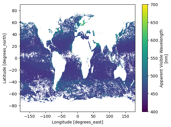
= ds["avw" ].sel(lat = slice (70 , - 70 )).mean(dim= ["lon" ])= "lat" );
Multiple months
= xr.open_mfdataset(= 'nested' , concat_dim= "time"
<xarray.Dataset> Size: 207MB
Dimensions:  (time: 8, lat: 1800, lon: 3600, rgb: 3, eightbitcolor: 256)
Coordinates:
  * lat      (lat) float32 7kB 89.95 89.85 89.75 89.65 ... -89.75 -89.85 -89.95
  * lon      (lon) float32 14kB -179.9 -179.9 -179.8 ... 179.8 179.9 180.0
Dimensions without coordinates: time, rgb, eightbitcolor
Data variables:
    avw      (time, lat, lon) float32 207MB dask.array<chunksize=(1, 512, 1024), meta=np.ndarray>
    palette  (time, rgb, eightbitcolor) uint8 6kB dask.array<chunksize=(1, 3, 256), meta=np.ndarray>
Attributes: (12/62)
    product_name:                      PACE_OCI.20240301_20240331.L3m.MO.AVW....
    instrument:                        OCI
    title:                             OCI Level-3 Standard Mapped Image
    project:                           Ocean Biology Processing Group (NASA/G...
    platform:                          PACE
    source:                            satellite observations from OCI-PACE
    ...                                ...
    cdm_data_type:                     grid
    identifier_product_doi_authority:  http://dx.doi.org
    identifier_product_doi:            10.5067/PACE/OCI/L3M/AVW/3.0
    data_bins:                         3016790
    data_minimum:                      399.99997
data_maximum: 700.00006 Dimensions: time : 8lat : 1800lon : 3600rgb : 3eightbitcolor : 256
Coordinates: (2)
Data variables: (2)
avw
(time, lat, lon)
float32
dask.array<chunksize=(1, 512, 1024), meta=np.ndarray>
long_name : Apparent Visible Wavelength units : nm valid_min : 400.0 valid_max : 700.0 reference : Vandermeulen, R. A., Mannino, A., Craig, S.E., Werdell, P.J., 2020: 150 shades of green: Using the full spectrum of remote sensing reflectance to elucidate color shifts in the ocean, Remote Sensing of Environment, 247, 111900, https://doi.org/10.1016/j.rse.2020.111900, https://doi.org/10.5067/KAROCHG01RYJ display_scale : linear display_min : 450.0 display_max : 575.0
Bytes
197.75 MiB
2.00 MiB
Shape
(8, 1800, 3600)
(1, 512, 1024)
Dask graph
128 chunks in 25 graph layers
Data type
float32 numpy.ndarray
3600 1800 8
palette
(time, rgb, eightbitcolor)
uint8
dask.array<chunksize=(1, 3, 256), meta=np.ndarray>
Bytes
6.00 kiB
768 B
Shape
(8, 3, 256)
(1, 3, 256)
Dask graph
8 chunks in 25 graph layers
Data type
uint8 numpy.ndarray
256 3 8
Indexes: (2)
PandasIndex
PandasIndex(Index([ 89.94999694824219,   89.8499984741211,              89.75,
         89.6500015258789,  89.55000305175781,  89.44999694824219,
         89.3499984741211,              89.25,   89.1500015258789,
        89.05000305175781,
       ...
       -89.05000305175781,  -89.1500015258789,             -89.25,
       -89.35000610351562, -89.45000457763672, -89.55000305175781,
        -89.6500015258789,             -89.75, -89.85000610351562,
       -89.95000457763672],
dtype='float32', name='lat', length=1800)) PandasIndex
PandasIndex(Index([ -179.9499969482422, -179.85000610351562,             -179.75,
       -179.64999389648438,  -179.5500030517578,  -179.4499969482422,
       -179.35000610351562,             -179.25, -179.14999389648438,
        -179.0500030517578,
       ...
         179.0500030517578,  179.15000915527344,              179.25,
        179.35000610351562,  179.45001220703125,   179.5500030517578,
        179.65000915527344,              179.75,  179.85000610351562,
        179.95001220703125],
      dtype='float32', name='lon', length=3600))
Attributes: (62)
product_name : PACE_OCI.20240301_20240331.L3m.MO.AVW.V3_0.avw.0p1deg.nc instrument : OCI title : OCI Level-3 Standard Mapped Image project : Ocean Biology Processing Group (NASA/GSFC/OBPG) platform : PACE source : satellite observations from OCI-PACE temporal_range : 27-day processing_version : 3.0 date_created : 2025-03-06T17:06:41.000Z history : l3mapgen par=PACE_OCI.20240301_20240331.L3m.MO.AVW.V3_0.avw.0p1deg.nc.param l2_flag_names : ATMFAIL,LAND,HILT,HISATZEN,STRAYLIGHT,CLDICE,COCCOLITH,LOWLW,CHLWARN,CHLFAIL,NAVWARN,MAXAERITER,HISOLZEN,NAVFAIL,FILTER,HIGLINT time_coverage_start : 2024-03-05T00:08:58.000Z time_coverage_end : 2024-04-01T02:24:44.000Z start_orbit_number : 0 end_orbit_number : 0 map_projection : Equidistant Cylindrical latitude_units : degrees_north longitude_units : degrees_east northernmost_latitude : 90.0 southernmost_latitude : -90.0 westernmost_longitude : -180.0 easternmost_longitude : 180.0 geospatial_lat_max : 90.0 geospatial_lat_min : -90.0 geospatial_lon_max : 180.0 geospatial_lon_min : -180.0 latitude_step : 0.1 longitude_step : 0.1 sw_point_latitude : -89.95 sw_point_longitude : -179.95 spatialResolution : 11.131949 km geospatial_lon_resolution : 11.131949 km geospatial_lat_resolution : 11.131949 km geospatial_lat_units : degrees_north geospatial_lon_units : degrees_east number_of_lines : 1800 number_of_columns : 3600 measure : Mean suggested_image_scaling_minimum : 450.0 suggested_image_scaling_maximum : 575.0 suggested_image_scaling_type : LINEAR suggested_image_scaling_applied : No _lastModified : 2025-03-06T17:06:41.000Z Conventions : CF-1.6 ACDD-1.3 institution : NASA Goddard Space Flight Center, Ocean Ecology Laboratory, Ocean Biology Processing Group standard_name_vocabulary : CF Standard Name Table v36 naming_authority : gov.nasa.gsfc.sci.oceandata id : 3.0/L3/PACE_OCI.20240301_20240331.L3b.MO.AVW.V3_0.nc license : https://science.nasa.gov/earth-science/earth-science-data/data-information-policy/ creator_name : NASA/GSFC/OBPG publisher_name : NASA/GSFC/OBPG creator_email : data@oceancolor.gsfc.nasa.gov publisher_email : data@oceancolor.gsfc.nasa.gov creator_url : https://oceandata.sci.gsfc.nasa.gov publisher_url : https://oceandata.sci.gsfc.nasa.gov processing_level : L3 Mapped cdm_data_type : grid identifier_product_doi_authority : http://dx.doi.org identifier_product_doi : 10.5067/PACE/OCI/L3M/AVW/3.0 data_bins : 3016790 data_minimum : 399.99997 data_maximum : 700.00006
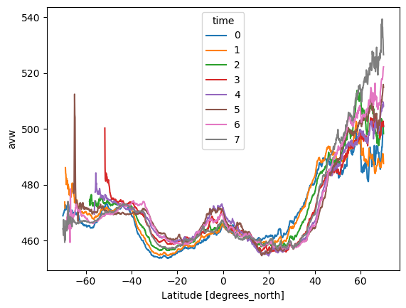
= ds["avw" ].sel(lat = slice (70 , - 70 )).mean(dim= ["lon" ])= "lat" );
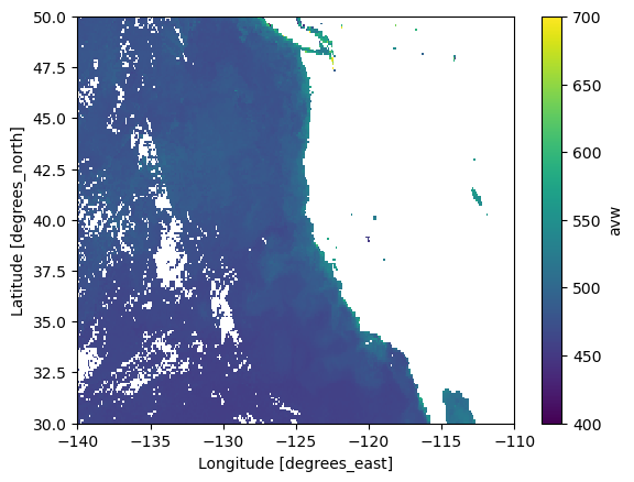
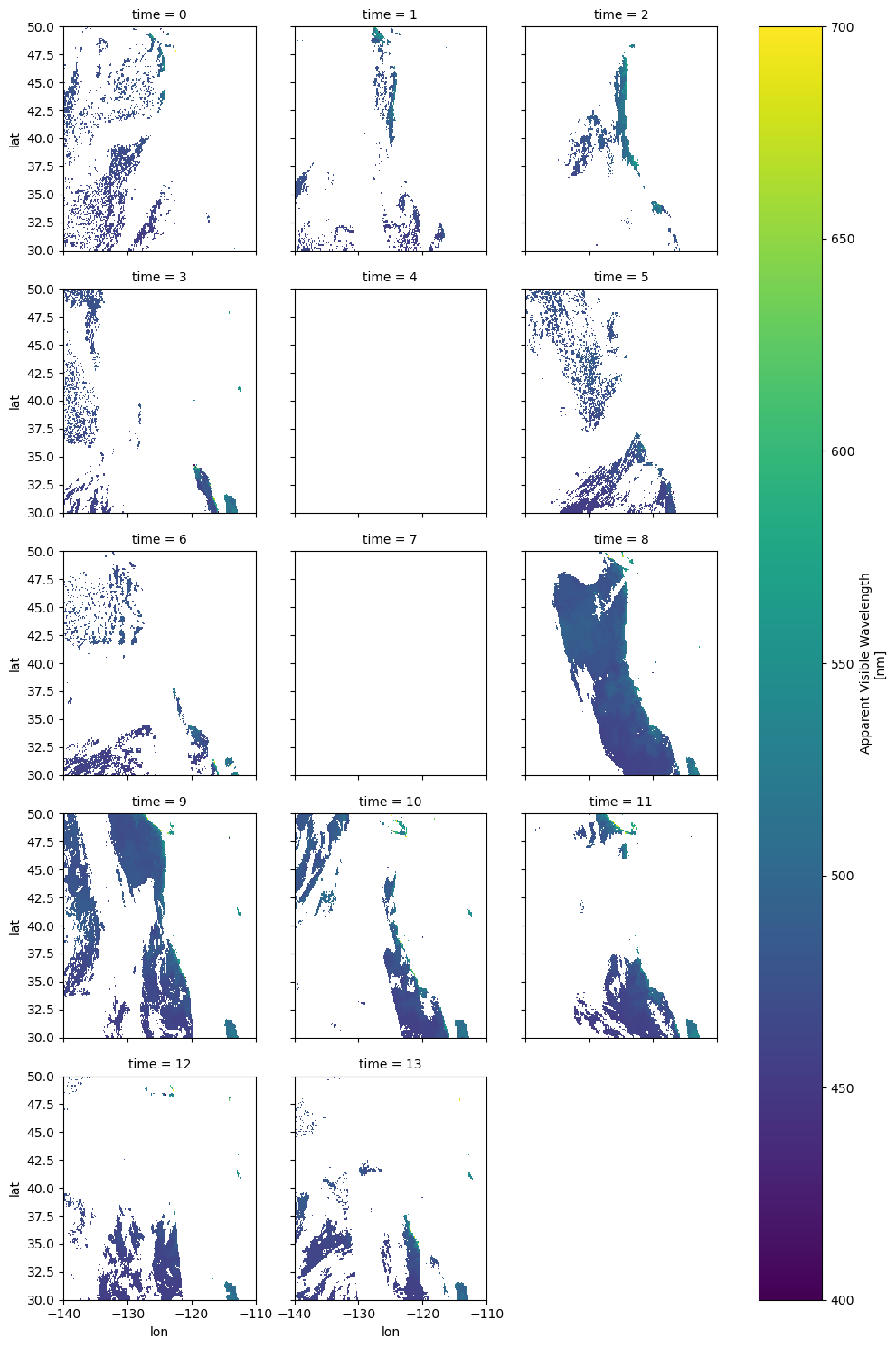
Daily data
We need the data links that have 0.1 deg and DAY in the file name.
import earthaccess= earthaccess.search_data(= "PACE_OCI_L3M_AVW" ,= ("2024-03-01" , "2024-03-31" ),= "*.DAY.*.0p1deg.*" len (results_day)
# let's load the data = earthaccess.open (results_day)
= xr.open_mfdataset(= 'nested' , concat_dim= "time"
<xarray.Dataset> Size: 363MB
Dimensions:  (time: 14, lat: 1800, lon: 3600, rgb: 3, eightbitcolor: 256)
Coordinates:
  * lat      (lat) float32 7kB 89.95 89.85 89.75 89.65 ... -89.75 -89.85 -89.95
  * lon      (lon) float32 14kB -179.9 -179.9 -179.8 ... 179.8 179.9 180.0
Dimensions without coordinates: time, rgb, eightbitcolor
Data variables:
    avw      (time, lat, lon) float32 363MB dask.array<chunksize=(1, 512, 1024), meta=np.ndarray>
    palette  (time, rgb, eightbitcolor) uint8 11kB dask.array<chunksize=(1, 3, 256), meta=np.ndarray>
Attributes: (12/62)
    product_name:                      PACE_OCI.20240305.L3m.DAY.AVW.V3_0.avw...
    instrument:                        OCI
    title:                             OCI Level-3 Standard Mapped Image
    project:                           Ocean Biology Processing Group (NASA/G...
    platform:                          PACE
    source:                            satellite observations from OCI-PACE
    ...                                ...
    cdm_data_type:                     grid
    identifier_product_doi_authority:  http://dx.doi.org
    identifier_product_doi:            10.5067/PACE/OCI/L3M/AVW/3.0
    data_bins:                         571271
    data_minimum:                      399.99997
data_maximum: 700.0001 Dimensions: time : 14lat : 1800lon : 3600rgb : 3eightbitcolor : 256
Coordinates: (2)
Data variables: (2)
avw
(time, lat, lon)
float32
dask.array<chunksize=(1, 512, 1024), meta=np.ndarray>
long_name : Apparent Visible Wavelength units : nm valid_min : 400.0 valid_max : 700.0 reference : Vandermeulen, R. A., Mannino, A., Craig, S.E., Werdell, P.J., 2020: 150 shades of green: Using the full spectrum of remote sensing reflectance to elucidate color shifts in the ocean, Remote Sensing of Environment, 247, 111900, https://doi.org/10.1016/j.rse.2020.111900, https://doi.org/10.5067/KAROCHG01RYJ display_scale : linear display_min : 450.0 display_max : 575.0
Bytes
346.07 MiB
2.00 MiB
Shape
(14, 1800, 3600)
(1, 512, 1024)
Dask graph
224 chunks in 43 graph layers
Data type
float32 numpy.ndarray
3600 1800 14
palette
(time, rgb, eightbitcolor)
uint8
dask.array<chunksize=(1, 3, 256), meta=np.ndarray>
Bytes
10.50 kiB
768 B
Shape
(14, 3, 256)
(1, 3, 256)
Dask graph
14 chunks in 43 graph layers
Data type
uint8 numpy.ndarray
256 3 14
Indexes: (2)
PandasIndex
PandasIndex(Index([ 89.94999694824219,   89.8499984741211,              89.75,
         89.6500015258789,  89.55000305175781,  89.44999694824219,
         89.3499984741211,              89.25,   89.1500015258789,
        89.05000305175781,
       ...
       -89.05000305175781,  -89.1500015258789,             -89.25,
       -89.35000610351562, -89.45000457763672, -89.55000305175781,
        -89.6500015258789,             -89.75, -89.85000610351562,
       -89.95000457763672],
dtype='float32', name='lat', length=1800)) PandasIndex
PandasIndex(Index([ -179.9499969482422, -179.85000610351562,             -179.75,
       -179.64999389648438,  -179.5500030517578,  -179.4499969482422,
       -179.35000610351562,             -179.25, -179.14999389648438,
        -179.0500030517578,
       ...
         179.0500030517578,  179.15000915527344,              179.25,
        179.35000610351562,  179.45001220703125,   179.5500030517578,
        179.65000915527344,              179.75,  179.85000610351562,
        179.95001220703125],
      dtype='float32', name='lon', length=3600))
Attributes: (62)
product_name : PACE_OCI.20240305.L3m.DAY.AVW.V3_0.avw.0p1deg.nc instrument : OCI title : OCI Level-3 Standard Mapped Image project : Ocean Biology Processing Group (NASA/GSFC/OBPG) platform : PACE source : satellite observations from OCI-PACE temporal_range : day processing_version : 3.0 date_created : 2025-02-14T03:36:43.000Z history : l3mapgen par=PACE_OCI.20240305.L3m.DAY.AVW.V3_0.avw.0p1deg.nc.param l2_flag_names : ATMFAIL,LAND,HILT,HISATZEN,STRAYLIGHT,CLDICE,COCCOLITH,LOWLW,CHLWARN,CHLFAIL,NAVWARN,MAXAERITER,HISOLZEN,NAVFAIL,FILTER,HIGLINT time_coverage_start : 2024-03-05T00:08:58.000Z time_coverage_end : 2024-03-06T02:07:24.000Z start_orbit_number : 0 end_orbit_number : 0 map_projection : Equidistant Cylindrical latitude_units : degrees_north longitude_units : degrees_east northernmost_latitude : 90.0 southernmost_latitude : -90.0 westernmost_longitude : -180.0 easternmost_longitude : 180.0 geospatial_lat_max : 90.0 geospatial_lat_min : -90.0 geospatial_lon_max : 180.0 geospatial_lon_min : -180.0 latitude_step : 0.1 longitude_step : 0.1 sw_point_latitude : -89.95 sw_point_longitude : -179.95 spatialResolution : 11.131949 km geospatial_lon_resolution : 11.131949 km geospatial_lat_resolution : 11.131949 km geospatial_lat_units : degrees_north geospatial_lon_units : degrees_east number_of_lines : 1800 number_of_columns : 3600 measure : Mean suggested_image_scaling_minimum : 450.0 suggested_image_scaling_maximum : 575.0 suggested_image_scaling_type : LINEAR suggested_image_scaling_applied : No _lastModified : 2025-02-14T03:36:43.000Z Conventions : CF-1.6 ACDD-1.3 institution : NASA Goddard Space Flight Center, Ocean Ecology Laboratory, Ocean Biology Processing Group standard_name_vocabulary : CF Standard Name Table v36 naming_authority : gov.nasa.gsfc.sci.oceandata id : 3.0/L3/PACE_OCI.20240305.L3b.DAY.AVW.V3_0.nc license : https://science.nasa.gov/earth-science/earth-science-data/data-information-policy/ creator_name : NASA/GSFC/OBPG publisher_name : NASA/GSFC/OBPG creator_email : data@oceancolor.gsfc.nasa.gov publisher_email : data@oceancolor.gsfc.nasa.gov creator_url : https://oceandata.sci.gsfc.nasa.gov publisher_url : https://oceandata.sci.gsfc.nasa.gov processing_level : L3 Mapped cdm_data_type : grid identifier_product_doi_authority : http://dx.doi.org identifier_product_doi : 10.5067/PACE/OCI/L3M/AVW/3.0 data_bins : 571271 data_minimum : 399.99997 data_maximum : 700.0001
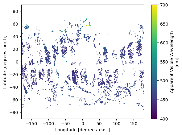
"avw" ].isel(time= 0 ).plot();
import matplotlib.pyplot as pltimport gc# Clear the current figure # Close the figure window # Ask Python to free up memory
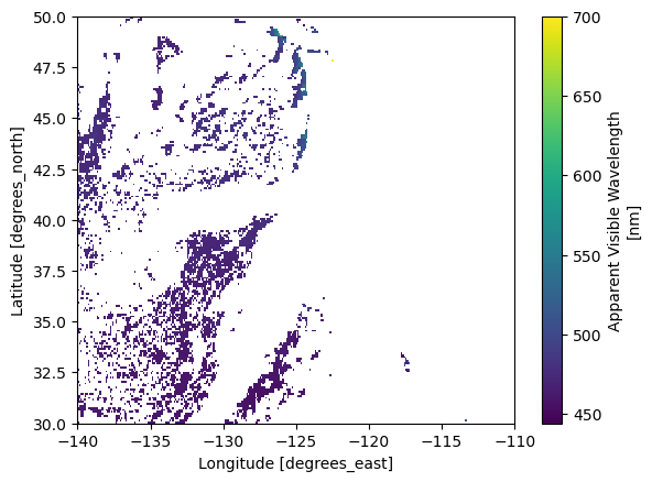
# let's look at the west coast of USA "avw" ].isel(time= 0 ).sel(lat = slice (50 , 30 ), lon= slice (- 140 , - 110 )).plot();
= ds["avw" ].mean(dim= "time" ); = slice (50 , 30 ), lon= slice (- 140 , - 110 )).plot();
# We can plot over the days to see when it was cloudy 'avw' ].sel(lat = slice (50 , 30 ), lon= slice (- 140 , - 110 )).plot(x= 'lon' , y= 'lat' , col= "time" , col_wrap= 3 );