Spectral phytoplankton absorption coefficients (APH)

Author

Eli Holmes (NOAA)

📘 Learning Objectives

Show how to work with the earthaccess package for PACE data

Create a NASA EDL session for authentication

Load single files with xarray.open_dataset

Load multiple files with xarray.open_mfdataset

Overview

The PACE Level-3 (gridded) OCI (ocean color instrument) data is available on an NASA EarthData. Search using the instrument filter “OCI” and processing level filter “Gridded Observations” https://search.earthdata.nasa.gov/search?fi=OCI&fl=3%2B-%2BGridded%2BObservations and you will see 45+ data collections. In this tutorial, we will look at the Spectral phytoplankton absorption coefficients (APH) product.

APH is in the IOP collection: PACE OCI Level-3 Global Mapped Inherent Optical Properties (IOP) Data, version 3.0. The concept id for this dataset is “C3385050632-OB_CLOUD” and the short name is “PACE_OCI_L3M_IOP”.

Prerequisites

You need to have an EarthData Login username and password. Go here to get one https://urs.earthdata.nasa.gov/

I assume you have a .netrc file at ~ (home). ~/.netrc should look just like this with your username and password. Create that file if needed. You don’t need to create it if you don’t have this file. The earthaccess.login(persist=True) line will ask for your username and password and create the .netrc file for you.

machine urs.earthdata.nasa.gov
        login yourusername
        password yourpassword

For those not working in the JupyterHub

Uncomment this line and run the cell:

# pip install earthaccess

Create a NASA EDL authenticated session

Authenticate with earthaccess.login().Authenticate with earthaccess.login(). You will need your EarthData Login username and password for this step. Get one here https://urs.earthdata.nasa.gov/.

import earthaccess
auth = earthaccess.login()
# are we authenticated?
if not auth.authenticated:
    # ask for credentials and persist them in a .netrc file
    auth.login(strategy="interactive", persist=True)

Import Required Packages

import xarray as xr

Monthly data

I poked around on the files on search.earthdata so I know what the files look like. March to December 2024.

import earthaccess
results_mo = earthaccess.search_data(
    short_name = "PACE_OCI_L3M_IOP",
    temporal = ("2024-03-01", "2024-12-31"),
    granule_name="*.MO.*aph.0p1deg.*"
)
len(results_mo)

results_mo[0]

Data: PACE_OCI.20240301_20240331.L3m.MO.IOP.V3_0.aph.0p1deg.nc

Size: 31.0 MB

Cloud Hosted: True

# Create a fileset
fileset = earthaccess.open(results_mo);

# let's load just one month
import xarray as xr
ds = xr.open_dataset(fileset[0])
ds

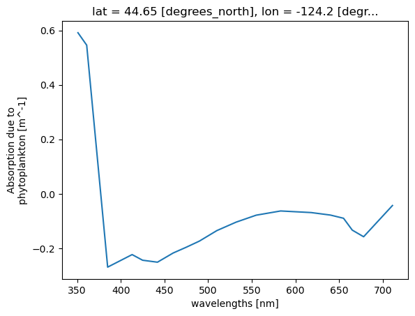
ds_np = ds['aph'].sel(lat=44.6517, lon=-124.1770, method='nearest')
ds_np.plot();

Multiple months

ds = xr.open_mfdataset(
    fileset,
    combine='nested', concat_dim="time"
)
ds

<xarray.Dataset> Size: 5GB
Dimensions:     (time: 10, lat: 1800, lon: 3600, wavelength: 19, rgb: 3,
                 eightbitcolor: 256)
Coordinates:
  * wavelength  (wavelength) float64 152B 351.0 361.0 385.0 ... 678.0 711.0
  * lat         (lat) float32 7kB 89.95 89.85 89.75 ... -89.75 -89.85 -89.95
  * lon         (lon) float32 14kB -179.9 -179.9 -179.8 ... 179.8 179.9 180.0
Dimensions without coordinates: time, rgb, eightbitcolor
Data variables:
    aph         (time, lat, lon, wavelength) float32 5GB dask.array<chunksize=(1, 16, 1024, 8), meta=np.ndarray>
    palette     (time, rgb, eightbitcolor) uint8 8kB dask.array<chunksize=(1, 3, 256), meta=np.ndarray>
Attributes: (12/64)
    product_name:                      PACE_OCI.20240301_20240331.L3m.MO.IOP....
    instrument:                        OCI
    title:                             OCI Level-3 Standard Mapped Image
    project:                           Ocean Biology Processing Group (NASA/G...
    platform:                          PACE
    source:                            satellite observations from OCI-PACE
    ...                                ...
    identifier_product_doi:            10.5067/PACE/OCI/L3M/IOP/3.0
    keywords:                          Earth Science > Oceans > Ocean Optics ...
    keywords_vocabulary:               NASA Global Change Master Directory (G...
    data_bins:                         3016341
    data_minimum:                      -0.7766001
    data_maximum:                      5.0000014

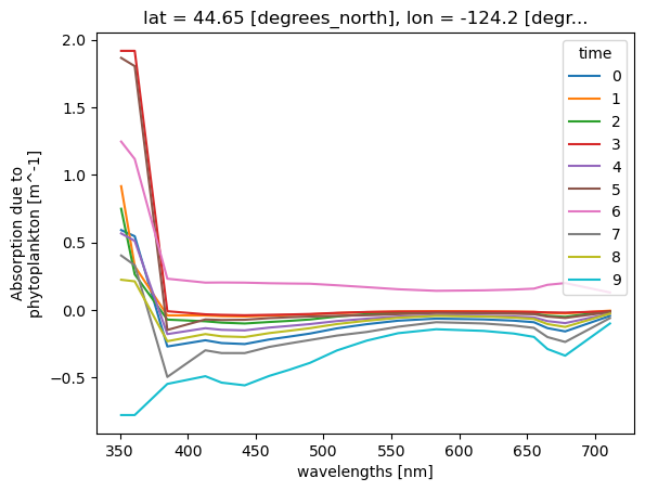
ds_np = ds['aph'].sel(lat=44.6517, lon=-124.1770, method='nearest')
ds_np.plot.line(x="wavelength");

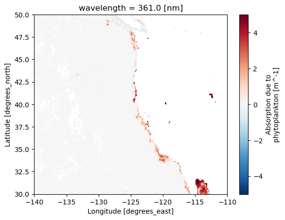
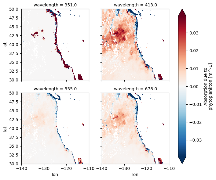
Raster plots of the APH

ds["aph"].isel(time=0).sel(wavelength = 361, lat = slice(50, 30), lon=slice(-140, -110)).plot();

ds["wavelength"].values

array([351., 361., 385., 413., 425., 442., 460., 475., 490., 510., 532.,
       555., 583., 618., 640., 655., 665., 678., 711.])

ds["aph"].isel(time=0).sel(
    lat=slice(50, 30), 
    lon=slice(-140, -110), 
    wavelength=[351, 413, 555, 678]  # choose your wavelengths
).plot(x="lon", y="lat", col="wavelength", col_wrap=2, robust=True);